CA Card
The CA card is used to define a section of a shielded cable which is used for irradiation (for example, computing induced currents and voltages at the cable terminals) due to external sources. Transmission line theory is applied, for example, no need to discretise the cable as with the MoM. A section is defined as a straight part of a cable (one cable can consist of multiple sections).
In the Solve/Run tab, in the Cables group,
click the ![]() Irradiating cable
(CA) icon.
Irradiating cable
(CA) icon.
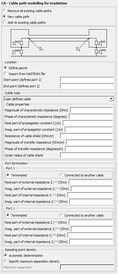
Parameters:
- Remove all existing cable paths
- If checked, all previously defined cable paths are removed. All the other input parameters are ignored.
- New cable path
- Defines a new cable path, all previously defined cable paths are replaced.
- Add to existing cable paths
- An additional cable path is defined (for example, the previously added ones will be kept).
- Location
- The location of the cable path section can be specified as two points or imported from
a NASTRAN file.
- Define points
- The Start point and the End point of the cable path section are defined by point names. These points must have been defined previously with a DP card (or by an external import).
- Import from NASTRAN file
- The name of the NASTRAN file and the property ID of the segments that have to be imported are required to import the cable path section.
- Cable type
- This specifies the type of cable. There are two possibilities: User defined cable or a
predefined cable from the internal Feko cable database:
- If User defined cable is selected
- The user has to enter all the cable properties in the Cable
properties section which will then be enabled. The units of the
individual parameters are included in the description. Note: That the Outer radius of cable shield will be scaled by any active SF card.Also keep in mind that most of these parameters may depend on the frequency and thus one might use variables or expressions.
- If a predefined cable type is selected
- The section containing the cable properties will be disabled, and all required parameters will be retrieved automatically from an internal Feko cable database. There are several commonly found shielded cable types (up to now all coaxial cables) included.
- Port termination
- This section is used to define the ports (for example, the two ends of the cable path section defined by this CA card). For each port the user can decide if it is terminated by an (internal and external) impedance or if this end of the cable path section shall be connected to another cable path section.
- Sampling point density
- The cable path section will be subdivided into small segments for the computation of the induced currents and voltages. The electric and magnetic field strengths will be evaluated at each segment’s centroid, so this setting influences the accuracy of the computed result, but also the computation time. The setting Automatic determination will choose the segment length automatically (which should be adequate for most cases). If the maximum separation distance is specified, then this value will override the automatic mechanism. Note that this manual value will be scaled by any active SF card.
Transmission line theory (TLT) is used in conjunction with the field calculation using the method of moments (MoM) to compute the voltage coupled-in at the termination impedances of a cable close to a conducting (metallic) ground. The cable itself is not taken into account when computing the external field distribution and it does not affect the field distribution at all, for example from a field-viewpoint of the scenario, the cable is not present at all. This is also the reason for the reduced number of unknowns in comparison to a full MoM solution: the cable itself is not modelled in the geometry and therefore not meshed into (wire) segments and it is therefore not necessary to introduce a very fine mesh on the ground plane underneath the cable. A further advantage of the transmission line approach is that multiple cable scenarios can be investigated in the same model (for example, different cable positions) without repetition of a time-consuming solution of the whole model (for example, MoM or MLFMM). Analysing another cable is similar to computing the near field at another point.

The term cable path refers to the complete cable from its start point to its end point. Thus the cable path can consist of a single or multiple cable path sections. Each cable path section is then again subdivided into the segments which are used for the computation. Each complete cable path has to be terminated on both ends.
An arbitrary number of cable path sections can be defined. The complete scenario is shown in Figure 2. It consists of the cable path connecting two (virtual) enclosures with the termination impedances. The cable is illuminated by an external electromagnetic field (as caused by sources and other radiating structures in the model) which couples into the cable and causes the currents and voltages in the internal termination impedances. For the calculation to work properly the segment direction vector and the ground vector must be (almost) perpendicular. This figure also shows the cable path, the cable path sections (1 . .. N) and the segments.

Figure 3 shows the setup of a number of cable paths. There are three cable paths in total (distinguished by the line style):
| Path | Description |
|---|---|
| 1 | Cable path from point 1 to 4 consisting of the cable path sections A, B, C. |
| 2 | Cable path from point 5 to 4 consisting of the cable path sections D, E, F, G. |
| 3 | Cable path from point 8 to 9 consisting of the single cable path section H. |
As the cable paths will be assembled automatically by searching and matching the points’ coordinates, the order of the CA cards determines how the cable path gets built. (The search is always started at the first CA card defining a termination impedance and then the cards will be processed in the order they appear in the input file.) For example, in order to get the situation as shown in Figure 3 the CA cards have to be in the following order:
- CA Defining section A (start cable path 1).
- CA Defining section B (continue cable path 1).
- CA Defining section C (end cable path 1).
- CA Defining section D (start cable path 2).
- CA Defining section E (continue cable path 2).
- CA Defining section F (continue cable path 2).
- CA Defining section G (end cable path 2).
- CA Defining section H (single segment cable path 3).
or (note the changed relative cable path number):
- CA Defining section A (start cable path 1).
- CA Defining section C (continue cable path 1).
- CA Defining section B (end cable path 1).
- CA Defining section H (single segment cable path 2).
- CA Defining section E (start cable path 3).
- CA Defining section D (continue cable path 3).
- CA Defining section F (continue cable path 3).
- CA Defining section G (end cable path 3).
but not in the following order:
- CA Defining section A (start cable path 1).
- CA Defining section B (continue cable path 1).
- CA Defining section D (end cable path 1).
- CA Defining section H (single segment cable path 2).
- CA Defining section E (start cable path 3).
- CA Defining section C (continue cable path 3).
- CA Defining section F (continue cable path 3).
- CA Defining section G (end cable path 3).
In the last case the cable path section D will be connected to the cable path section B which is not intended! (Cable path 1 would then start at point 1 and end at point 5 consisting of sections A, B, D and cable path 3 will then start at point 4 and end at point 4 consisting of the sections C, E, F, G.) Additionally in this case the cable path 3 will form a closed loop, but one has to keep in mind, that even in this case the two ends of the cable path are not connected at point 4.
Current limitations of the cable irradiation analysis using the CA card:
- For the built-in cable types, the frequency range is limited as this data is based on measurements only available for a certain frequency range. Currently the frequency range from 10 kHz up to 500 MHz is supported for all those cable types. (An error is given by Feko if one tries to set a frequency which is not in that range.) This restriction is not applied for user defined cables, since it is assumed that the user has supplied the required cable parameters for the frequency under consideration.
- The cable must be homogeneous, for example, the cable parameters may not vary for the sections belonging to the same cable path (this is enforced for all cables).
- Currently only single conductor coaxial cables are supported. A multi-conductor cable cannot be modelled.
- Cables cannot be used in connection with UTD, but any other method is possible to represent the external configuration (for example, a car body modelled with MoM or MLFMM).
- A reference plane acting as ground is required for the cable coupling algorithm. This is currently implemented in such a way that only metallic triangles and perfectly conducting ground planes (PEC-ground defined by a BO-card) are considered. Feko will give an error if the special Green’s functions are used in connection with a cable analysis.
- Connections of cables with wires or crossings with wires are not allowed. Even if a cable path starts or ends at a point where also a wire segment starts or ends or if a cable path crosses a wire, there will be no electrical connection established between the cable and the wire at such a point.