View Field

Implicit modeling represents geometry as a 3D field of scalar values. In general, positions where the field is equal to zero are on the surface of the object. By convention, negative scalar values are inside the object, and positive scalar values are outside the object.

It is not always easy to imagine the underlying field of an implicit body, especially after several operations have been performed on that field. The View Field setting enables users to visualize the underlying field for an implicit object using contours and a colormap. This tool is most effective when used with a Section Plane so the interior of an object can also be viewed.

Let's now consider an illustrative workflow. In this model, we created a sphere and a cube that overlap. We then used a Boolean Combine operation to make them one object, followed by a Remap operation to reconstruct the correct signed distance field.

The resulting object looks like this:

If we activate the View Field option, the following is displayed.

Although this is correct, a more meaningful scene is shown if we use a Section Plane on the part:

In the image above, red regions are external to the object, blue regions are internal, and black contours/surfaces are on the surface. White contours are used like a 3D ruler to show how the scalar values of the field are progressing away from the surface.

Let us now look at the controls in the View Field guide panel in more detail.

The Field Values controls let us set the field values of interest that will be colored and contoured by the View Field tool. For example, we may only be interested in field values +/-10mm from the surface. This can be achieved with the following settings:

We now only have color and contours spanning the relevant field values, and the rest of the scene is blank.

It is also useful to be able to change the Reference Value for the field. By default, this is set to zero, which is the surface of the object. However, if we wanted to visualize what the surface would look like with an inward offset of 10 mm, we could change the reference field value to -0.01 m:

We now have the black contour at the location of the offset surface. The blue regions of the colormap are no longer visible, as there are now field values within the Min Value and Max Value range that fall on the interior of the newly specified Reference Value. This is a key point: the colormap colors field values less than the reference value in blue, and field values greater than the reference value in red. For the rest of the demonstration, we will adjust the field Min Value and Max Value settings to color the entire volume.

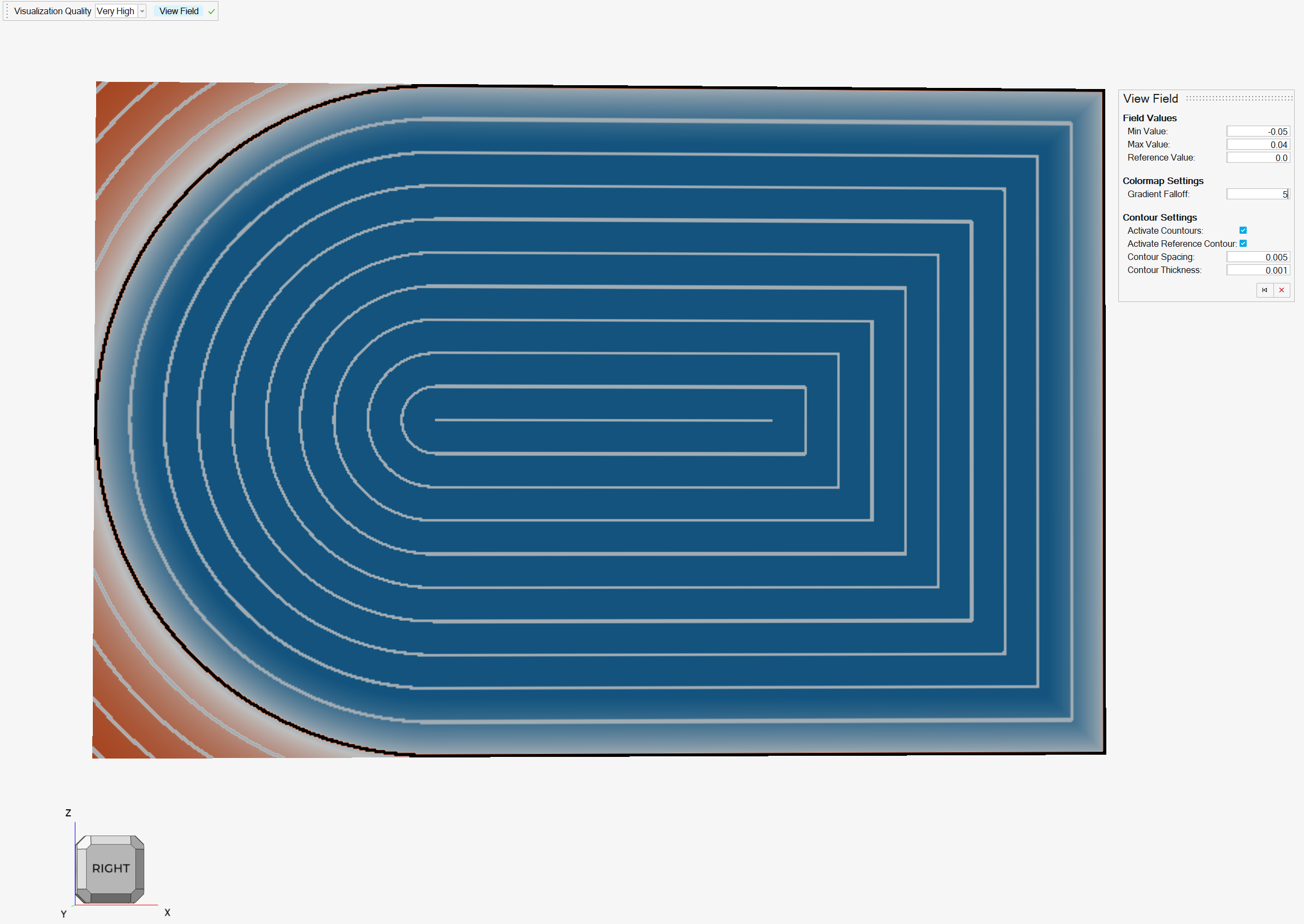
Depending on the field, the gradient in the colormap may not be as illustrative as we might want. We can control how quickly the colormap gradient moves from red to white (near Reference Value contour) to blue. The following examples show different stylings by changing the Gradient Falloff in the Colormap Settings. The first image is a Gradient Falloff of 0, the second is a Gradient Falloff of 5, and the third image is a Gradient Falloff of -1 (any negative value forces block coloring with no gradient). As a useful aside, setting the Gradient Falloff to 0 means that gradient is linearly proportional to the scalar value change, which is useful for signed distance fields.

The next group of settings come under the Contour Settings heading . The black contour is reserved for the Reference Value in the field that is specified by the user. The white contours represent isocontours that progress away from the reference value at a given spacing.

First, we will look at the different visual effects that are created by (de)activating various contours.

Once you have selected a preferred visual style, you can edit the contour thickness and spacing for any active contours. The images below show some different examples. The first image uses a large contour spacing.

We can reduce the contour spacing to see more contours.

If the contour lines are too thick, we can make them thinner.

Alternatively, we can make the contour lines thicker.