
Thinking in Fields - A Primer for Implicit Modeling
A detailed description of how fields are used in Implicit Modeling within Inspire, with videos and illustrative examples that will help you think intuitively in terms of field-driven design.
Most Computer-Aided Design (CAD) represents a 3D object by describing the surfaces that enclose it (i.e., a "boundary representation (BRep)"). This includes parametric surfaces (e.g., NURBS), tessellated surface meshes (e.g., planar triangles), and subdivision surfaces. Implicit modeling is not a BRep; it is a volumetric representation. It represents geometry as a field, which encodes information about every position in space that is external to an object, and every position in space that is internal to an object. The surface itself is implied as the boundary between the external and internal regions in space.
What Do We Mean When We Say "Field"?
The term field means different things to different people and different disciplines.
For clarity, within the context of Implicit Modeling, the term field takes the following definition: at every coordinate in a space, usually within some practical bounds, the field returns a signed scalar value (e.g., 1.0, -3.1, 0.0, etc.). We use field as a shortening of the more complete term, scalar field. The information encoded by the field is of the form {x-coordinate, y-coordinate, z-coordinate, signed scalar value}.
Implicit Modeling makes use of some important conventions within the context of geometry. Firstly, negative scalar values are assumed to be internal to the modeled object, and positive scalar values are external. The surface of the object, itself, appears at every location in space that returns a scalar value of zero. As such, the signed scalar values in the field give an immediate inside/outside check for any coordinate in space.
The following paragraphs describe the different types of fields that are useful in Implicit Modeling and that fall within the scope of this definition.
Different Types of Fields
Descriptions of the different types of fields that are useful in Implicit Modeling and that fall within the scope of this definition.
Signed-Distance Fields (SDFs)
SDFs are particularly useful as they give instant inside/outside checks, and they tell you how close a point is to the surface of an object. This arrangement is optimal for creating accurate offset surfaces for a given geometry, and they also enable controlled blending between surfaces, filleting operations, and much more.
Unsigned Distance Fields (UDFs)
UDFs share all of the same properties as SDFs with one clear exception: all scalar values in the field have the same sign (+/-), irrespective of whether they are internal or external to the object being modeled. Some geometries produce UDFs by construction, such as lines, curves, and points. This is because there is no well-defined notion of inside and outside for these objects. However, it can sometimes be useful to construct an UDF in place of an SDF. This is achieved by taking the absolute value of the SDF, producing all positive distances.
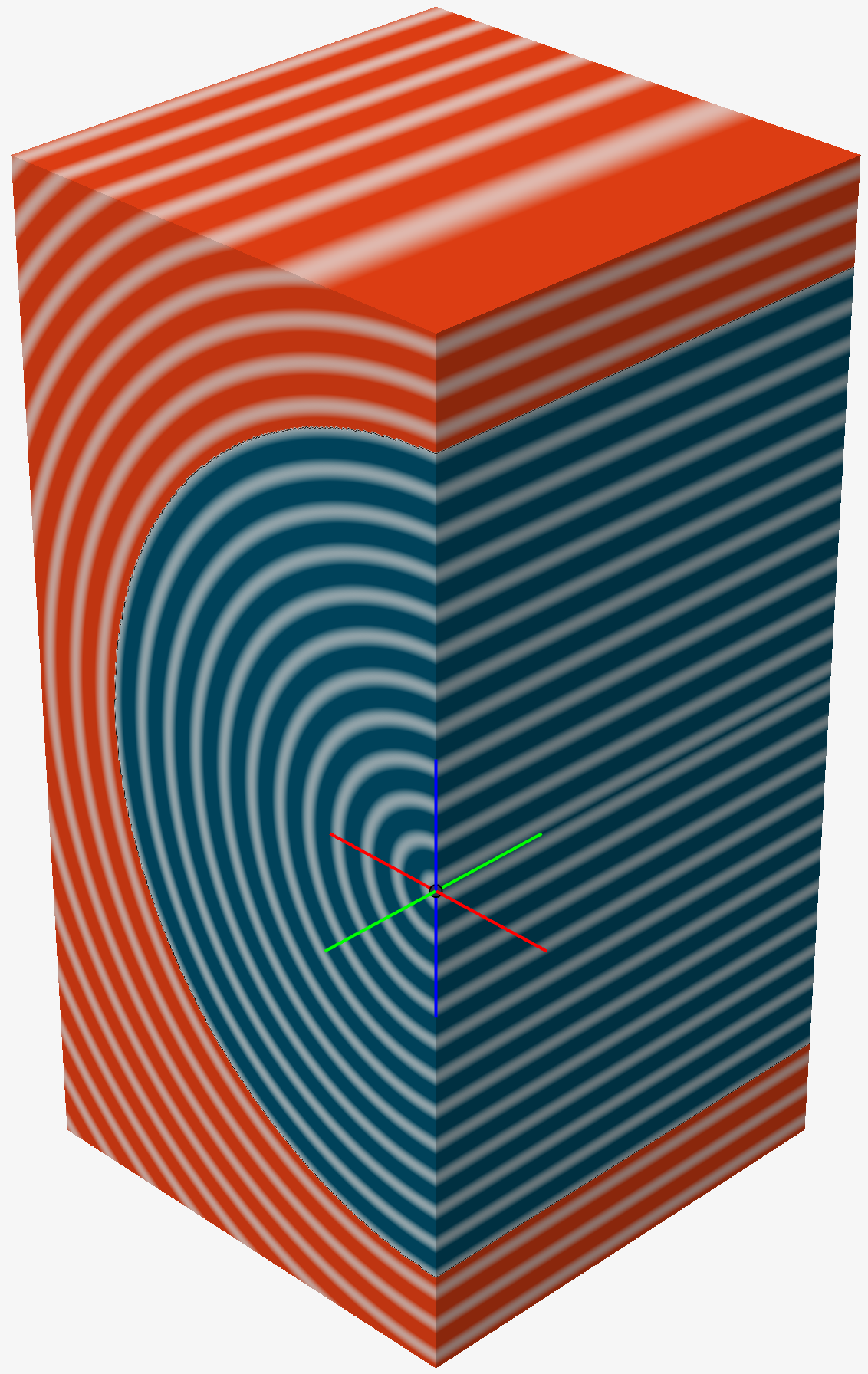
Distance-Like Scalar Fields
Binary and Piecewise Constant Fields
It is possible to create binary fields, which, by convention, are zero everywhere outside and on the surface and one everywhere inside of the surface of an object. These fields can be very useful for masking off regions in space to limit the scope of a downstream operation. For example, you might wish to apply geometry edits strictly within certain regions without applying them elsewhere. This is like saying “perform an operation in all of these positions, but do not perform the operation anywhere else.”
Similar to binary fields, it can be useful to create constant fields. Typically, these fields have one user-defined value inside and on the object, and either the same or a different user-specified values outside of the object. For example, you could create a field that has scalar values of 3 inside and on the surface of the object and a value of 5 outside the object. These fields can be useful for setting, for example, thicknesses of lattice elements in different regions.
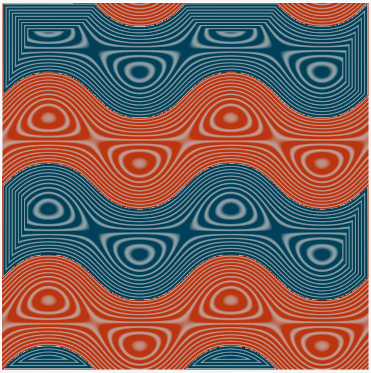
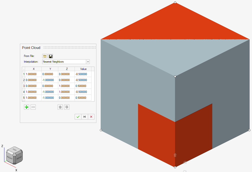
Interpolating Scalar Fields
- Simulation data
- Measurement data
- Sampled values from a mathematical function
- Knowledge from previous experience
Inverse Distance Weighting

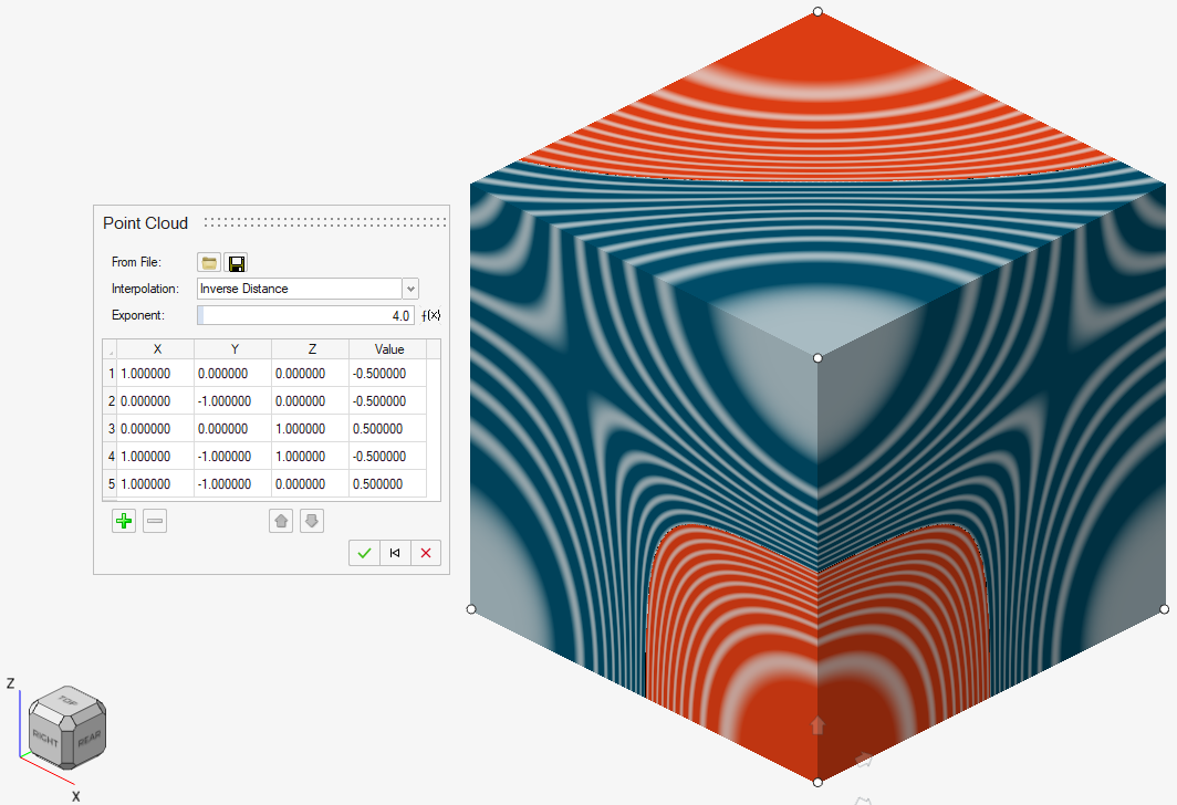
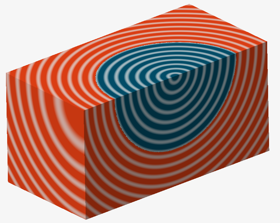
Nearest Neighbor Interpolation
Nearest Neighbor interpolation is simpler to visualize. Each position in the field adopts the scalar value of the nearest point in the point cloud. This technique forces abrupt changes in the resulting Interpolating Scalar field as nearby positions in space may "snap" to different scalar values.
Using Fields to Create Shapes
Fields can be used to create geometry by extracting the isosurface that passes through all positions in space where the field is equal to zero.
The following simple example explains how this works.
In 3D Cartesian coordinates, a popular equation for a sphere is
,
where are the center coordinates of the sphere and is the radius.
However, to represent the sphere as a SDF, we present the equation of the sphere in the following format:
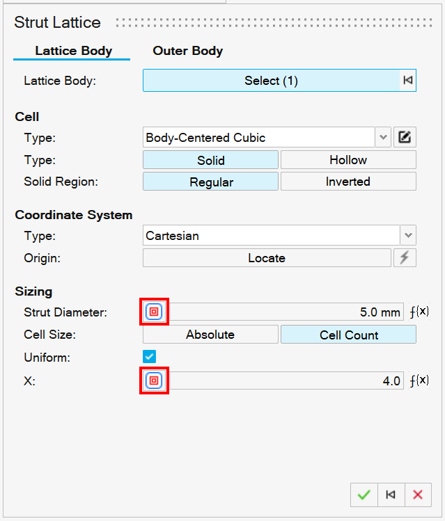
Field-Driven Design: Using Fields to Edit Properties of Existing Shapes
Fields can be used to locally vary certain parameters or sizings for existing geometry.
For examples, please see Video Tutorial: Creating Field-Driven Effects in Lattices.
Here is a simple example of field-driven design.
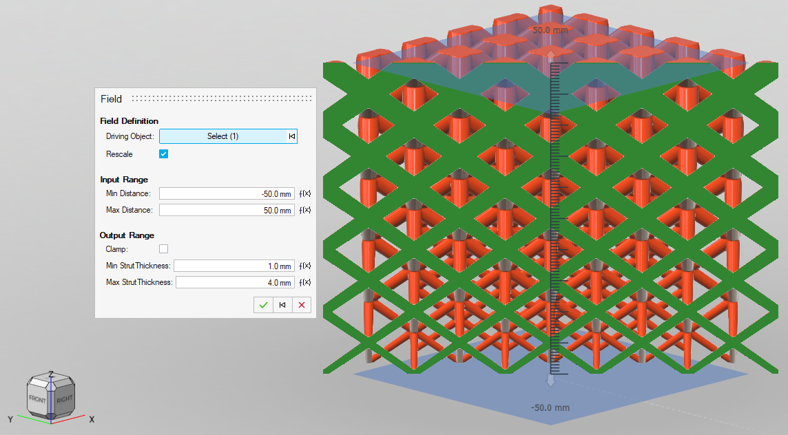
- Relating the local thickness of a lattice or shell to structural simulation data, thereby carefully placing material where it is needed
- Automatically controlling the radius of fillets throughout a model based on the level of stress experienced in that location, thereby efficiently relieving local stress raisers
- Locally strengthen or weaken structures to deliberately route forces through a preferred path (e.g., safely absorbing impact)
- Locally altering the sizing of lattice structures to changes non-structural properties (e.g., electromagnetic behavior, permeability or pressure drop in fluid flow, acoustic performance, heat-transfer coefficients, etc.)
- Seamlessly merge from one geometry type to another, to create different (meta) material properties in specific locations (e.g., morph from one lattice type to another to exploit their respective advantages within the same object)
Misconceptions and Pitfalls of Implicit Modeling
Some common and not-so-obvious misconceptions and pitfalls when working with implicit modeling.
Some Common Misconceptions and Pitfalls When Working with Implicit Modeling
"I'm used to working with sketches."
Traditional CAD workflows tend to start with 2D sketches that get developed into 3D features using a handful of tools that loosely map onto manufacturing processes (extrude, revolve, etc.). Implicit Modeling is different in that it builds shapes up by defining, combining, and blending between volumetric (3D) shape representations from the beginning. If you need to develop your model from sketches, you should follow a traditional CAD workflow and then convert your model into an Implicit format when the time is right.
"Why can't I click on individual features?"
Traditional CAD, driven by NURBS surfaces, explicitly defines the surfaces that envelop the modeled object. The trimming lines for each surface that form well-defined boundaries between surfaces and features are also available by construction. Implicit Modeling has no such features, and they cannot be readily selected, highlighted, or edited. This is because the entire surface of the object is a single isosurface, implied as the boundary between the interior and exterior regions of the object's field. It is therefore difficult to select points on a surface, lines that separate features, and isolated faces. For the time being, this is the price that is paid for the additional flexibility in terms of creating complex, robust, and field-driven geometry.
"Why isn't there a dimension tool?"
As Implicit modeling is not sketch, feature, and constraint driven (like traditional CAD), a dimensioning tool is limited in its usefulness. Instead, geometry sizing and positions should be entered carefully at the point of creation, possibly controlled by a variable or field for added flexibility.
"I want to convert/export my Implicit Modeling to Parametric CAD (NURBS)."
Almost every geometry representation can be converted into an Implicit format with little difficulty. This conversion process outputs a SDF for the object. However, Implicit geometry cannot always convert back to other formats as easily. Implicit geometry is easy to mesh and can be output as .stl, .obj, and .3mf formats. You should be mindful that very complex implicit models might produce dense meshes with very high triangle counts. The route back to parametric CAD is via the PolyNURBS tool. This tool can be used to fit subdivision surfaces to the Implicit model, making them editable CAD surfaces. Again, care should be taken during these steps, as you will be trading off computing time and accuracy during the fitting process. Parametric CAD is a poor choice for a very complex model, as their will be too many surfaces to handle the model efficiently.
"Why do sharp edges look rounded?"
Although many fields technically have infinite resolution, they ultimately end up being sampled using a 3D grid. The coarseness or fineness of this grid is controlled by the Visualization Quality. Were the grid to be infinitely fine, sharp edges would be perfectly sharp. As the grid becomes coarser to match the computing resources available, sharp edges become somewhat rounded in both rendering and any subsequent conversion to, for example, a triangle mesh.
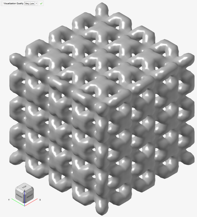
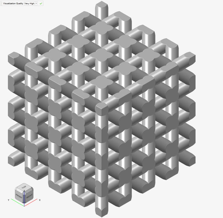
To minimize this effect, you should finish the design in the highest visualization quality that your computer can tolerate, possibly even using a custom quality.
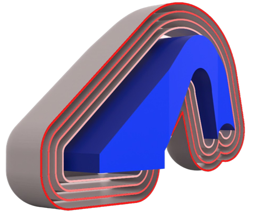
A Not So Obvious Pitfall: Not All Implicit Modeling Operations Preserve Distances When Combining SDFs
A common operation in implicit modeling is to combine separate bodies to form one connected body. This is often referred to as a Boolean union operation, but implicit modeling uses the shorter term "Combine." One would be forgiven for thinking that combining two bodies, each represented by an SDF, would result in another SDF. However, let's take a look at what happens to the field in this case. The images below were created using the following steps:
- Create two cuboid primitives that are offset from each other but still overlapping.
- Combine the objects (Boolean union).
- Create an inward shell of the combined object to create a hollow object of constant wall thickness.
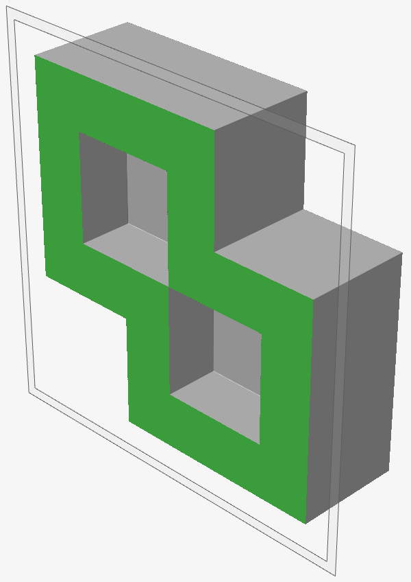
Careful inspection of the above images will show that the wall thickness is not constant. Specifically, the region where the wall thickness causes the internal corners to touch represents a wall thickness that is larger than expected.
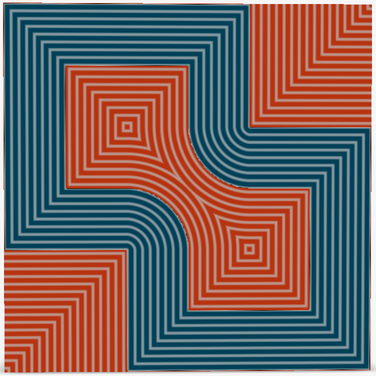
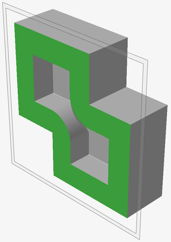
To summarize, simply combining multiple SDFs does not necessarily result in a SDF after the operation. The same is true of other operations, such as smoothing, morphing, and offsetting operations. It is useful to keep this in mind when using Implicit Modeling in general.
Concluding Remarks For Field-Driven Design
You have now had an introduction to what is going on behind the scenes in Inspire Implicit Modeling. Keeping this information in mind when working with the application will enable you to exploit the major benefits of Implicit Modeling, including field-driven design, while avoiding some of the common pitfalls.
Specific information on how to use each of the tools within the Implicit Modeling ribbon are given throughout the rest of the Implicit Modeling documentation.