
Point Clouds in Implicit Modeling
To drive a field or create implicit geometry, you can import a point cloud or create one from scratch.
Many of the contexts in Inspire Implicit Modeling permit you to drive the properties of a geometry with a field. Examples include changing the relative density or thickness of a lattice, or the radius of a fillet at different points in space. If the field used to control this sizing is defined from geometry, this is very straightforward. However, you often only know about the sizing requirements at specific points in space. The sizing elsewhere is less strict and can be generated automatically using different interpolation techniques, drawing influence from nearby locations where information is supplied. This scenario is handled using the Point Cloud context in Implicit Modeling.
The Point Cloud context asks you to provide data at known locations in space by specifying the x-, y-, and z-coordinate of each point, and also the scalar value of the field at that point. Point cloud data in this format can be imported from a .csv file or created from scratch using the user interface. The scalar values could be derived from simulation results, known quantities based on engineering experience, driven by an equation, etc. For every position in a field that is not represented explicitly by a point in the cloud, the scalar value is created automatically using interpolation. Example interpolation techniques include Inverse Distance Weighting and Nearest Neighbor interpolation.
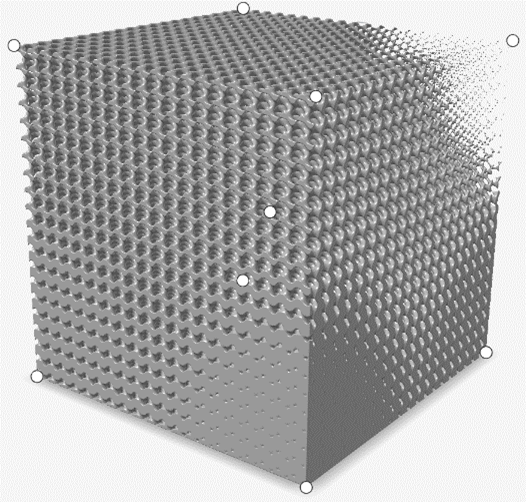
Inverse Distance Weighting behaves much like gravitation. For example, a point particle positioned between the earth and the moon would experience the gravitational effects of both the earth and the moon. The contribution of gravitation from the earth and the moon depends on the position of the point particle relative to both bodies, and the strength of the gravitational field from each body at that location. The same is true in Inverse Distance Weighting interpolation, where the influence of each of the cloud’s points (and their respective scalar values) at a certain position in space depends on the distance to each point in the cloud and the sign and magnitude of the scalar values. In the example image, below, Inverse Distance weighting has been used to smoothly interpolate the known relative density values of the lattice that have been specified at the point locations.
Nearest Neighbor interpolation is simpler to imagine. Each position in the field adopts the scalar value of the nearest point in the point cloud. This technique forces abrupt changes in the resulting Interpolating Scalar field as nearby positions in space might "snap" to different scalar values.
By default, the field created by the points in the point cloud are purely based on the interpolated values of each point. However, it is possible to assign a background value to the point cloud so that the points modify an already existing value or field. The points will have a radius and falloff factor associated with them so they have an area of influence and smoothing factor that allows a user to sculpt the background value or field.
Create a Point Cloud
You can import a .csv file or build a point cloud from scratch. When modifying the point cloud, you can change the number and position of points, the interpolation strategy and, for Inverse Distance Weighting interpolation, the exponent. You can save the point cloud as a .csv file.
When creating a point cloud to generate implicit geometry, keep in the mind that the main concept in implicit modeling is to represent a surface as the zero level set of an implicit function. This function takes a point in 3D space as input and returns a scalar value. Points with values near zero are considered part of the surface, while points with positive or negative values are outside or inside the surface, respectively.
-
On the Implicit Modeling ribbon, select the
Point Cloud tool.

Tip: To find and open a tool, press Ctrl+F. For more information, see Find and Search for Tools. - Optional: For Visualization Quality, select from Low to Very High quality, which corresponds to a low to very high density of elements. A higher quality produces sharper geometry features but is more computationally intensive. When creating a complicated function, it’s recommended to work using a lower quality and then switch to a higher quality after the function is complete.
- Optional:
To
import a point cloud:
-
In the Point Cloud dialog box, click the Import
icon.

- Browse to the .csv file.
- Click Open.
The table is filled with data. -
In the Point Cloud dialog box, click the Import
icon.
-
Select a type of Interpolation.
- Inverse Distance: The scalar value at a position that is not specified in the point cloud data is computed as the weighted average of scalar values of points in the point cloud. The weighting with respect to each point in the point cloud is a function of the distance to each point in the cloud. Scalar values at a point specified in the point cloud data will be exactly equal to the supplied scalar value.
- Nearest Neighbors: The scalar value at a position that is not specified in the point cloud data is equal to the scalar value of the closest point in the cloud.
- Define the Exponent, which can be a constant value or variable. This is a number greater than or equal to one. Smaller values propagate the effect of a point farther through space and larger values make the effect of a particular point's scalar value more localized around that point.
- Choose whether the field created by the point cloud will produce a Distance field or if is going to be used as a Utility function to be used as a field-driven function for another implicit parameter. The main difference this choice makes is whether the point cloud will try to be rendered as geometry or not.
- Optional:
Assign a background value to the point-cloud field.
- Enable the Background Value checkbox.
- Assign a constant value, variable, or field to the background value
- Select whether the values generated by the points will Bump the background value, or use the Set option to ensure the resulting field will have values that exactly pass through the values at each point while interpolating through the background value.
-
Create a point cloud from scratch or modify the existing one:
To Do this Reposition a point Adjust the X, Y, and Z coordinates and the Value. Add a new point Click the + sign and enter the X, Y, and Z coordinates and Value. Delete an existing point Select the row, and then click –. Reposition a row Select the row, and then click the up or down arrow. -
To save the point cloud:
-
Click the Save icon.

- Browse to the desired folder.
- Enter the file name.
- Click Save.
-
Click the Save icon.
- Click OK.
- Generate a continuous surface representation from point cloud data to create implicit geometry. For example, you could heal topology optimization data where there's a dimple that you want to remove. You could take the union of the topology optimization field and a point cloud field to fill it in.
- Create a field with the point cloud as the driving object. You can then map the parameters of an implicit object to the field driven by the point cloud. For example, the scalar values in a point cloud may relate to stress data from a simulation. For this illustrative example, assume this data lies in the range of 1 kPa to 5 kPa, depending on the point's location. If this data is used to create a field that controls the radius of the beams in a strut lattice, these values need to be rescaled to lie in the range of thicknesses that are well-suited to these values. Continuing with this example, you might know that regions experiencing stress of 1 kPa should have a thickness of 1mm and regions experiencing stress of 5kPa require a thickness of 5 mm. The rescale feature in the Field context should be used to map the range of stresses into the range of strut diameter (i.e., 1 kPa maps to 1 mm and 5 kPa maps to 5mm). Note that these values are only for illustration purposes and you should use values appropriate for your application.