Create a Field For Implicit Modeling

Create a field to define geometry or control the parameters of an existing geometry at every location within the bounds of the field.

In implicit modeling, the spatial properties of geometry can be controlled using a field. This might apply to the relative density of a lattice, making it locally thicker or thinner at different positions. It can also apply to other modification commands, such as fillets and shell/offset amounts, giving locally larger or smaller fillet radii and shell/offset thicknesses.

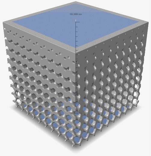
A field can be thought of as a 3D grid, and each grid point contains a signed scalar value. An illustrative example would be to create a field based on the signed distance to a plane or line, and then rescale these distances into density values. This field can then be used to control the relative density of another geometry, such as a lattice, at each location in space.

You can construct a field from a source that is not yet described in a field format and remap field values to different ranges.

1. On the Implicit Modeling ribbon, select the Field tool.
   
   
2. Optional: For Visualization Quality, select from Low to Very High quality, which corresponds to a low to very high density of elements. A higher quality produces sharper geometry features but is more computationally intensive. When creating a complicated function, it’s recommended to work using a lower quality and then switch to a higher quality after the function is complete.
3. Select a driving object.
   Note: The driving object can be an implicit body; reference geometry such as points, planes, and axes; or a selection of BRep geometry types such as vertices, straight edges, arcs, and planar and cylindrical faces. Information that is already in a field format can be used, such as simulation data (e.g., stress fields), which includes data in the form of a point cloud if interpolation is used.
   The driving object is converted into the correct field format. For geometry, this creates a 3D grid of coordinates and then creates a scalar value for each coordinate. In almost all cases, this will be the signed distance to the object from the point of view of that coordinate. For an existing field, it will look up and/or interpolate the existing field values to place them into the newly created 3D grid of coordinates and corresponding scalar values.
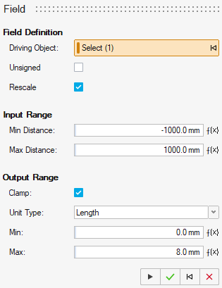
4. Optional: To map the distance field to a new output range, turn on Rescale.
   An illustrative example is to control the relative density of a lattice based on the signed distance values. Here, signed distance values will be rescaled into the desired relative density range. For example, if you want a relative density of 25% at zero distance to the driving geometry and a relative density of 75% at 50 mm away from the object, the inputs to the rescale will be as follows:

   Min Distance: 0.0 mm

   Max Distance: 50.0 mm

   Min Density: 25.0

   Max Density: 75.0

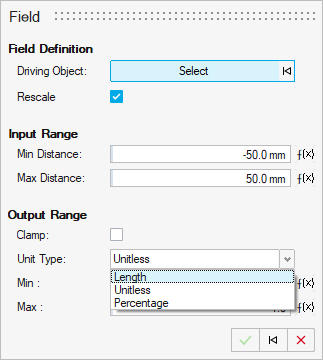
5. Define the Input Range, which can be constant or variable driven.
   • Min Value: The lowest numerical value of interest in the input field, which might come from driving geometry such as distance to an implicit body, distance to construction geometry (point, axis, and plane), or select BRep features (vertex, line segment, arc, planar surface, cylindrical surface). Please note that this is not the value that is closest to zero, it is the smallest value on a number line. For example, -25.3 is smaller than -0.1.
   • Max Value: The highest numerical value of interest in the input field, which might come from driving geometry such as distance to an implicit body, distance to construction geometry (point, axis, and plane), or select BRep features (vertex, line segment, arc, planar surface, cylindrical surface). Please note that this is not the value that is closest to zero; it is the largest value on a number line. For example, -0.1 is larger than -25.3.
6. Define the Output Range, which can be constant or variable driven.
   • Units: The units associated with the output field, which can either be Length, Unitless, or Percentage. Percentage is used for applications, such as the Relative Density of a lattice, which is expressed as being between 0% (empty space) and 100% (completely solid). Another example is the Morph Amount in the Morph context. Unitless is the correct choice for applications that are represented as a count, without any units. An example of this is specifying lattice unit cell sizes based on a count across one of the dimensions of an object (e.g., "give me 20 repetitions of the lattice unit cell in the x-direction").

     

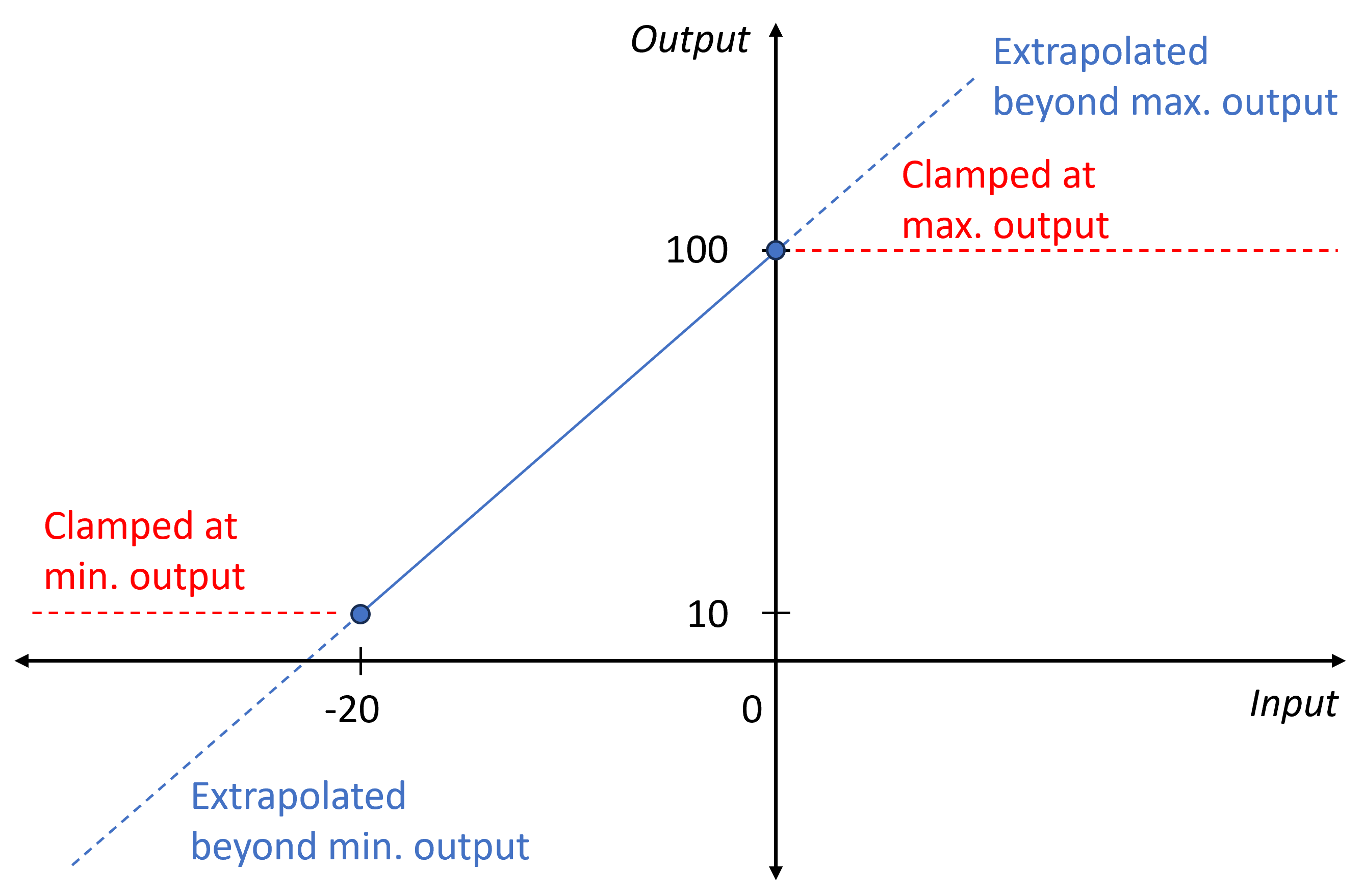
   • Min Value: The value that the Min Value from the input field should map to in the newly created output field (e.g., a density value of 25% or a distance such as 0.0 mm).
   • Max Value: The value that the Max Value value from the input field should map to in the newly created output field (e.g., a density value of 75% or a distance such as 50.0 mm).
7. Optional: To prevent values going below or above the Min and Max values, respectively, turn on Clamp.
8. Click OK.

Another way to think about Rescaling values in a field is to consider the following plot. In this illustrative example, the input ranges from a minimum value of -20 to a maximum value of 0. The output ranges from 10 to 100. The rescaling operation is a linear transformation that maps the input range to the output range (i.e., -20 maps to 10 and 0 maps to 100). The linear transformation can be thought of as the straight line graph that passes through these two points (solid blue circles). Between the minimum and maximum, values will vary linearly. Outside of minimum and maximum, one of two things will happen. If Clamp is deactivated, values will be linearly extrapolated unless a physical limit is reached (blue dashed lines). An example of a physical limit arises in relative density, where values cannot exceed 100% or go beneath 0%. If Clamp is activated, values outside of the limits will be fixed at the limit values, represented by red dashed lines in the plot.

The field is saved automatically and can be used to drive certain implicit parameters.