File Import Flux
Introduction
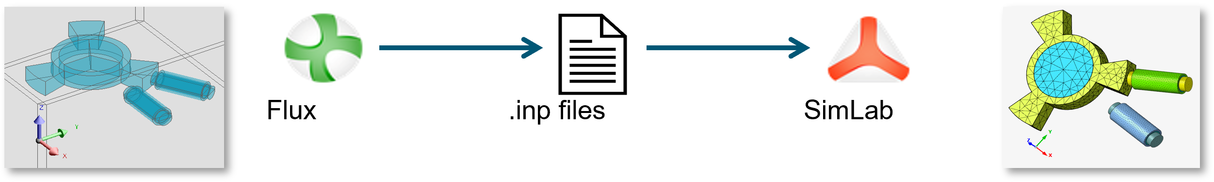
For legacy flux user, it's possible to import a Flux project into SimLab via Abaqus format.
Two workflows are still available:
- legacy workflow via in several steps starting from Flux (explained in this page below).
- new worflow since simLab 2026 directly in simLab via drag and drop of the flux
project or via the command .
 Note: All information is available in a new page Import Flux project.
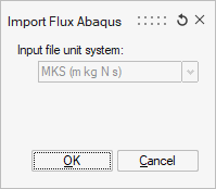
Dialog Box
This dialog has the options used in importing Flux input file.
Legacy Workflow
- Open the Flux project which you want export
- In the menu Project select
- Choose the Output directory
- Click on OK
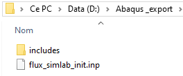
→ The main files flux_simlab_init.inp is created with a folder called includes containing all needed secondary files
→ Some internal modifications of Flux project are needed before to perform the Abaqus export (More detail about Flux project: required modifications).
Step 2 Result Step 4 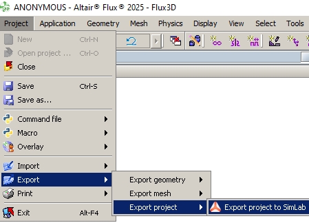
 Note: If the chosen directory is not empty, a message appear to propose to erase or the content of the directory (YES) or to choose another directory (NO → go to step 1, and choose another directory at the step 3))
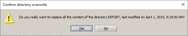
- Open SimLab
- Import the master abaqus file *.inp:
- Open the Import dialog box by selecting
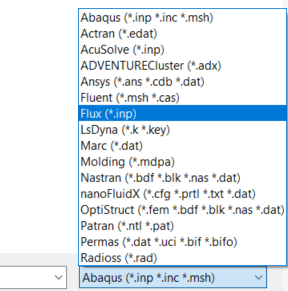
- Choose the extension of the import as Flux
(*.inp) in the bottom right corner:→ the folder is filtered and only the flux_simlab_init.inp is displayed
Step 6a Step 6b 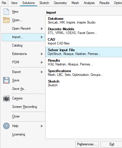
-
Select the file "flux_simlab_init.inp" and validate by clicking on OK.
→ a first dialog box "Import Flux Abaqus" is dispalyed only with the information of Input file unit system used.
Click on OK
→ Some Warnings could be displayed
→ The Flux project is imported in SimLab and the database SimLab is created with all corresponding Bodies, LBC,...→ A log is opened with the list of missing entities and other informations
-
Step 6c 6d 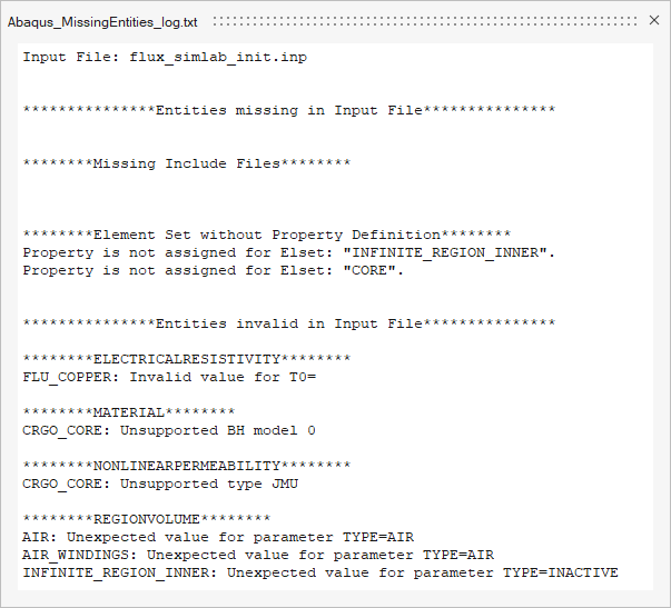
→ The log file "AbaqusImport_log.txt" is stored in the user scratch directory define in Preference of SimLab. By defaut it's:
C:\Users\"NameOfUser"\AppData\Local\Temp\SimLab\SimLab_2025\Temp\temp_x
