Liquid Cooling
![]()
Introduction
Liquid cooling is an ElectroFlo smart object used for defining the cooling liquid region with specific flow parameters.
Description
- Electronic components can have advanced cooling entities, such as liquid cooling, to avoid thermal damage.
- Liquid cooling smart object is used to define all the required liquid
cooling parameters combinedly in a single GUI.
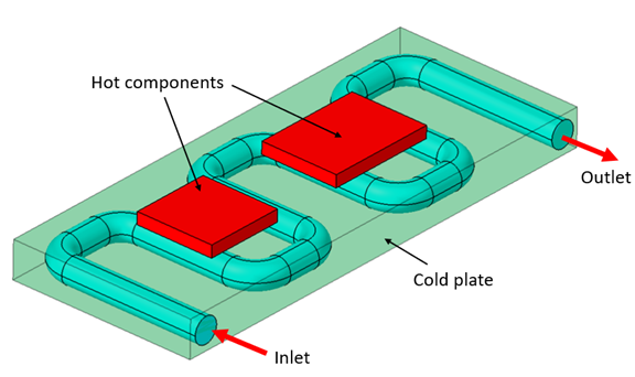
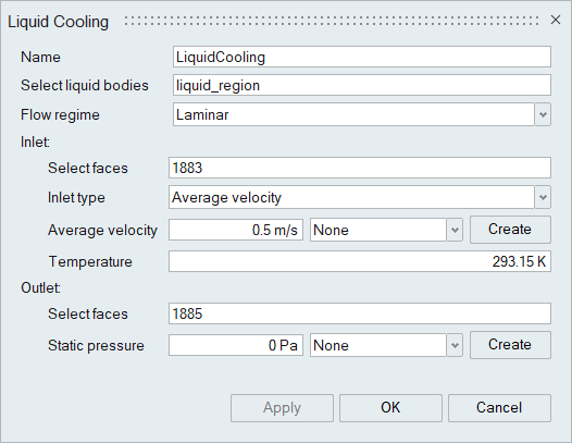
- User can define the liquid cooling region by selecting the bodies applied with “Fluid” materials.
- The Flow regime for the cooling liquid region can be set as,
- Laminar
- Turbulent
- Turbulent flow regime can be solved by the below methods.
- Standard K-epsilon
- Zero equation
- Spalart–Allmaras
- User can select the inlet face regions and define the Inlet parameters
as,
- Mass flow rate
- Volume flow rate
- Average flow velocity.
- Temperature must be also defined in the inlet region.
- Outlet pressure can be defined by selecting the outlet face region and entering the corresponding value in the “Static pressure” field.
- Inlet Flow parameters and outlet pressure can be either constant or variable
if a multiplier function is defined.
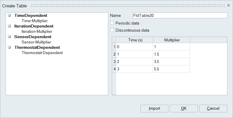
- There are three types of multiplier tables:
- Time - Multiplier value varies as a function of time in transient simulations.
- Iteration - Multiplier value varies as a function of the iteration number in steady-state simulations.
- Sensor – Multiplier value varies based on the selected sensor output.
- Thermostat - Multiplier value varies based on the ON/OFF status of the selected thermostat.
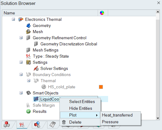
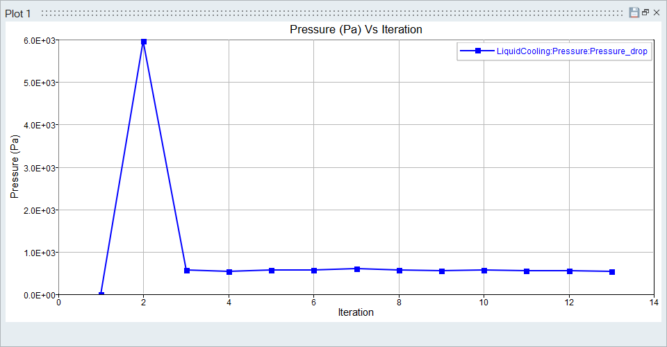
Graph Plotting
Pressure drop and Heat transfer parameters can be plotted by right click on “Liquid cooling” under “Smart Objects” in the solution browser.