Sheet Lamination

Analysis > Magnetic Transient Loads > Sheet Lamination

Introduction

The Sheet Lamination allows to define stacked magnetic sheets and allows to compute iron losses (only Bertotti model at this time).

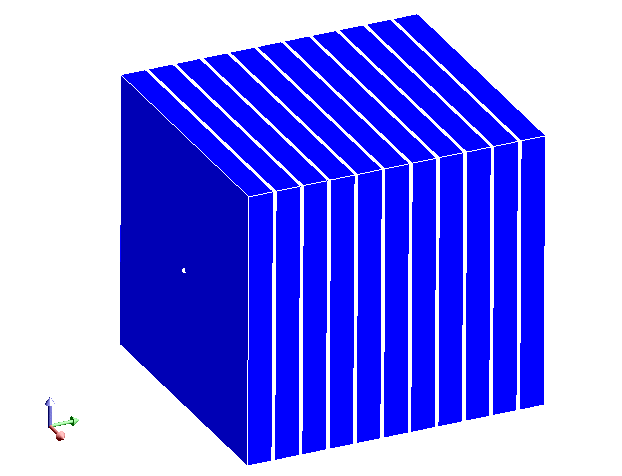
This Load enables the modeling of a laminated part: magnetic (permeability μ_r) non conducting, like stacked magnetic sheets simplified via the homogenization method.

With Sheet lamination load, there is not need to represent geometrically each sheet.

It is defined by:

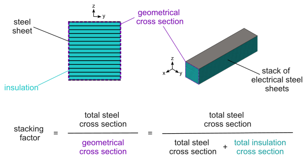
a stacking factor:
The sheet lamination is said to be laminated because it automatically accounts for the effect of the insulation of the electrical steel and for the small air gaps between the sheets in a stack. This is achieved through a homogenization procedure implemented. The overall effect of this homogenization is that the effective cross-section of magnetic material available for the magnetic flux to traverse in the region is reduced. The reduction factor is known as the stacking factor of the region, and corresponds to the total cross section area occupied by magnetic material (steel) in the stack divided by the surface area of the geometrical cross section of the same stack (i.e., the total cross section area, including the insulation and air gaps between sheets). This definition is illustrated below:

Sheet laminations are often used in magnetic circuits of transformers and of some electrical machines in order to reduce Eddy current losses. Here is an example of laminated transformer:

The eddy current distribution is shown on the following image for both Massive magnetic circuit and Laminated magnetic circuit:

Iron losses - principle

Magnetic losses (or iron losses) computation is an a posteriori computation, carried out in post-processor.

The power losses in electromechanical devices are mainly of three types:

the magnetic losses in the magnetic circuits (also called ‘iron losses’)
the losses by Joule effect in coils (also called ‘copper losses’)
the mechanical losses (mainly by friction in rotating machines)

Losses in magnetic materials:

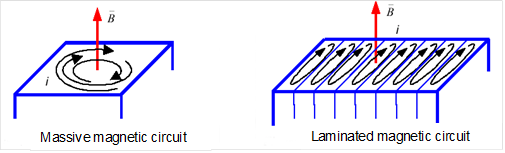
The power losses in magnetic materials are connected to the phenomena associated with the time variation of the magnetic field. They are subdivided into hysteresis losses (of microscopic origin) and Eddy current losses (of macroscopic origin). In fact, they are Eddy currents in both cases.

The hysteresis losses (microscopic Eddy currents) are associated to currents at a small scale. These currents are the result of local flux density variation caused by the magnetic structure in movement (essentially wall movement).
The Eddy losses (macroscopic Eddy currents), are due to the excitation frequency. They appear when domain wall displacement increases due to frequency increase.

Magnetic losses and hysteresis cycle:

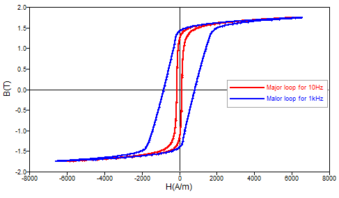
In practice, magnetic materials are characterized by their hysteresis cycle and the magnetic losses can be represented by this cycle, as presented below:

the volume energy created by hysteresis losses is corresponding to static hysteresis cycle (f<1Hz).
as the frequency increases, the cycle area increases and the volume energy created by Eddy current losses is corresponding to the difference between the dynamic hysteresis cycle area and the static one.

Iron losses computation in SimLab

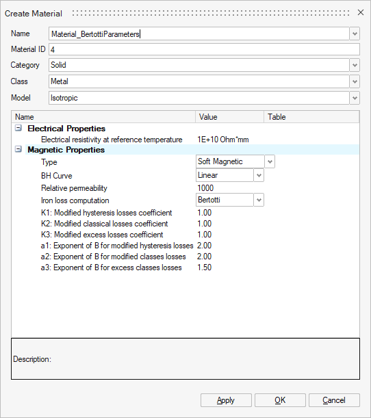
To be able to compute the iron losses in SimLab, the material assigned to the body defined by a sheet lamination load should be a soft magnetic material with 3 coefficients and 3 exponents of Bertotti Model.

For 2D and 3D Transient Magnetic solutions, in Result Request, in Sheet Lamination Results node, you should choose True for Iron Losses computation and define the min and max steps to define the exact electrical period.

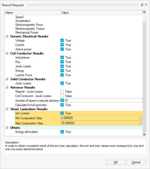Attention: In order to obtain physically meaningful results, the user must choose the correct time interval. The user must select a time interval corresponding to one and only one electrical period of the device.

Note: The first two time steps of a scenario can not be selected for the time interval definition and are hidden from the list.

Note: Flux solver interprets the provided time interval as a full electrical period. More specifically, Flux solver checks the periodicity of the magnetic flux density B(t) by comparing its values at the first and last time steps of the selected interval. Then, if the periodicity tests fail, Flux solver displays a warning message, but the computation is nevertheless carried out.

Modified Bertotti model for 2D and 3D Transient Magnetic solutions

With the modified Bertotti model, the iron loss density (directly related to the specific losses by the mass density) in a stack of electrical steel sheets may be decomposed in a sum of three terms: namely hysteresis, classical (also called eddy current) and excess losses terms. In each point of the material described by a laminated magnetic non conducting region, in the time domain the following equation holds:

where

represents the instantaneous iron loss density, in W/m³;
$λ_{F}$ is the stacking factor of the lamination;
$k_{1}$ is the hysteresis losses coefficient;
$α_{1}$ is the hysteresis losses exponent;
$k_{2}$ is the classical losses coefficient;
$α_{2}$ is the classical losses exponent;
$k_{3}$ is the excess losses coefficient;
$α_{3}$ is the excess losses exponent;
$T_{}$ is the period of the magnetic flux density;
and are the maximum excursions from their continuous component, of the longitudinal and the transversal projections of the homogenized magnetic flux density over the period $T_{}$ , respectively; in each point of the laminated region, the longitudinal direction is defined as the direction of $B_{}$ at the time step where the magnetic flux density reaches its maximum value during the considered period, while the transversal direction is orthogonal to the longitudinal one, as shown in the image below;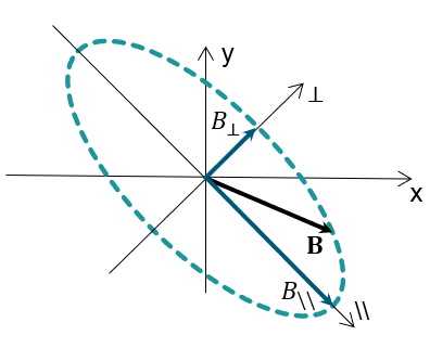
is the magnitude of the time derivative of the homogenized magnetic flux density, which has been beforehand decomposed into its longitudinal and transversal projections defined here above.

Sheet Lamination Dialog Box for 3D Transient Magnetic and 3D Magnetic AC solutions

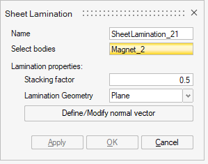
Select bodies: one or several bodies to define as sheet lamination.
Lamination properties:
- Stacking factor
- Lamination Geometry
  2 types:
  - Plane
    
    The direction of the planar sheet lamination is defined by a normal vector, by clicking on Define/Modify normal vector
  - Cylinder
    
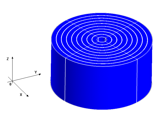
    The direction of the cylindrical sheet lamination is defined by the cylinder axis, by clicking on Define/Modify cylinder axis

Steps

Check the prerequisites:
1. a Soft Magnetic Material with Bertotti parameters should be assigned to the body
Click on the Sheet Lamination button in Analysis ribbon:
Select bodies: Select one or several bodies to define as a sheet lamination.
Choose the Stacking factor
In 3D, define the Lamination Geometry
Validate by clicking on OK
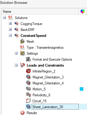
→ The sheet lamination is created and appears in the Solution Browser in the Loads and Constraints node.
Before solving, edit Result Request and define the Sheet Lamination Results
1. Choose True for the Iron Losses
2. For 2D and 3D Transient Magnetic solutions, define the interval: Min Computation Step and Max Computation Step
3. Validate by clicking on OK

Note: After finishing the modeling, you can solve and post-process the iron losses of each sheet lamination defined in EM Response or in a 2D Plot.