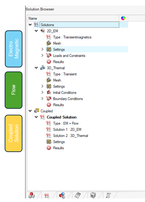
Coupled Solution: Electromagnetic + Flow
![]()
Introduction
- Strong coupling
At each time step, through iteration between Flux and AcuSolve, losses and temperature values are updated until convergence for temperature data is achieved.
This solution is slower as iterations are required, but more accurate especially when the magnetic solution is heavily dependent on temperature and heavily transient problems.
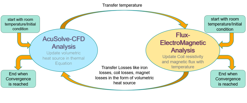
- Weak coupling
The process is the same as strong coupling, expect that only one iteration is performed, instead of iterating until convergence.
This method is faster and should give good results for steady states or slow transient coupling problems.
Power losses in electrical machines act as heat sources in thermal analysis. Temperature fluctuations influence material properties, resulting in reduced performance and lower output power. Specifically, iron and Joule losses, primarily calculated using the Flux Solver, are imported into the AcuSolve solver to serve as heat sources. In a Bidirectional Coupled Solution, the updated temperature is transferred back to the Flux Solver. This temperature feedback causes temperature-dependent materials to alter their properties, thereby impacting the power losses.
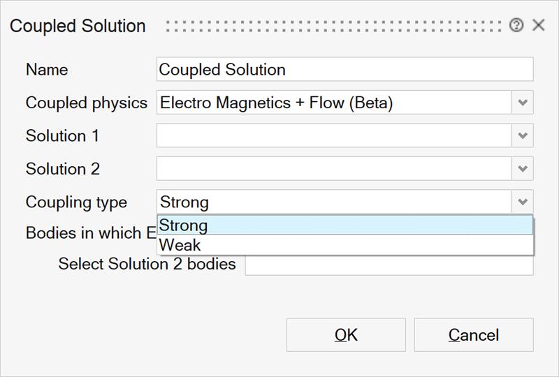
Dialog box
Simlab provide an easy method to define the coupling workflow.
For the Bidirectional (weather strong or weak) type, the following steps allow the easy creation of a Coupled Solution:
- Set up the Electromagnetic Solution.
- Set up the Flow Solution.
- Couple the Electromagnetic and the Flow solutions through the Coupled
Solution button and identify the bodies of the CFD model which
requires mapping of the heat losses.
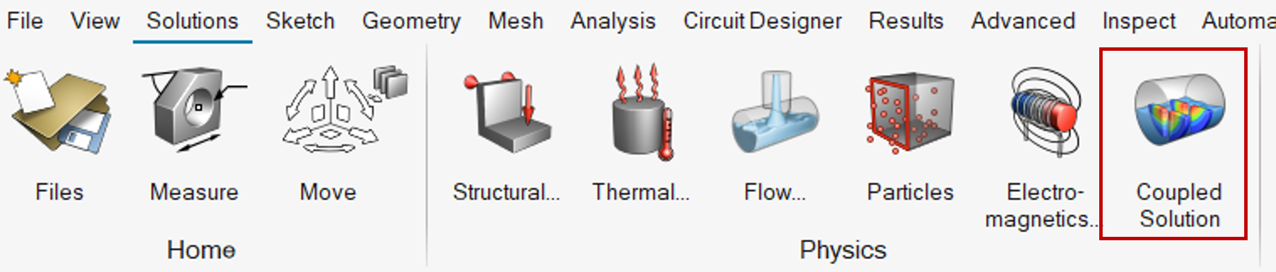
→ the dialog box "Coupled Solution is displayed
- Choose the Solution 1
- Choose the Solution 2
- Choose the Coupling type
- Select bodies
- Validate the coupled solution by clicking on
OK
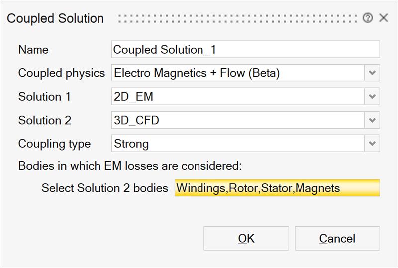
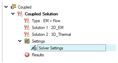
→ The solution browser should display 3 solutions : EM solution, CFD solution and the newly created coupled solution.
Settings
- Before creating the Coupled Solution, the user must validate the
following settings in the Electromagnetic Solution:
- Solution Window Settings
- Solution Type: MT2D, MT3D, MAC2D, MAC 3D are available. For MAC 2D and MAC 3D, only one step is possible, multi-position solutions are not available.
- Result Request SettingsIn the Advanced Results section:
- Averaged Joule Losses: set to True.
- Averaged Iron Losses: the user must select an electrical period.
- Iron losses set to
True: the user must select an
electrical period.Note: The Min. Computation Step always begins at the third step. The first two steps are ignored when computing Iron Losses. Therefore, it is necessary to add two extra steps to the Electromagnetic Solution to accommodate this behavior.Note: The materials used for laminated bodies are not temperature dependent. Therefore, even if the Averaged Iron Losses field is activated, the Iron Losses will not be updated based on changes in temperature.
Note: The fields Number of layers in extrude direction and Calculate for full geometry have no impact on the results of the Coupled Solution.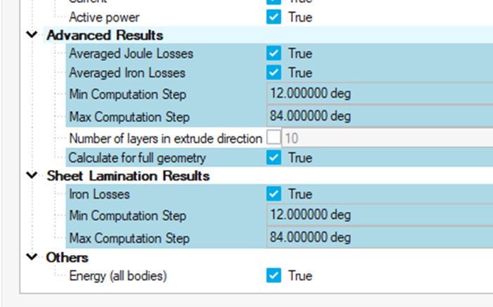
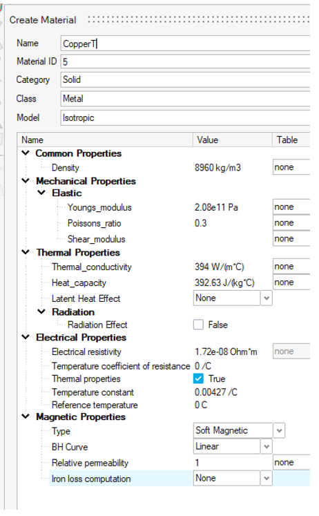
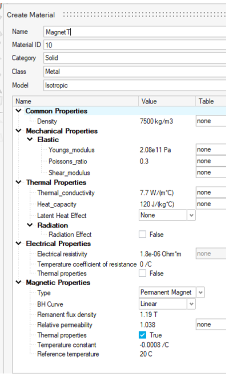
- For Joule Loss and Iron losses calculations, ensure that
the assigned materials have their Thermal
Properties enabled. This applies to materials like
CopperT and MagnetT, as shown in the following example screenshots.
- Solution Window Settings
- Before creating the Coupled Solution, the user must validate the
following settings in the Flow Solution:
- Solution Window Settings
- Solution Type: Ensure it is set to Transient
- Result Request Settings
- In the Nodal Output section, the Output time interval field must be filled with a numeric value. This numeric value could be the number of steps (Final time divided by Time step size defined in the Flow Solution)
- Solution Window Settings
- After creating the Coupled Solution:To finalize the Coupled Solution setup, validate or update solvers settings:
- Right-click on Settings
- Select Solver Settings
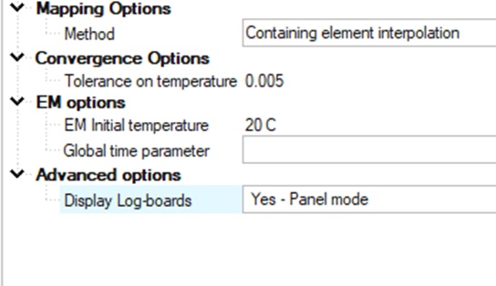
- Mapping options : defines the mapping method, default option is “Containing Element Interpolation”
- Convergence Option: set tolerance criteria
- EM options:
- EM Initial temperature is defined from CFD solution
- Global time parameter : Flux variable defining the global time parameter (same time as the CFD simulation), as opposed to the steps of the MT solution over which losses will be averaged. Typical application is when the rotation speed of the motor change over time. In this case, it can be defined as a function of a variable called “global-time”. During the co-simulation, at each new global time step, the new global time value will be updated in the Flux solution, the speed will then be different over the global time, but over an electric period represented by the Flux scenario and its TIME, the speed will remain constant.
- Click the OK button to confirmNote: settings can be left to defined values (with possible exception of global time depending on the loadcase).
Note: The Coupled Solution is driven by the Flow Solution. This means that the Final time and Time step size defined in the Flow Solution will also serve as the time settings for the Coupled Solution.