Temperature
![]()
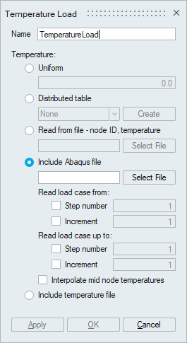
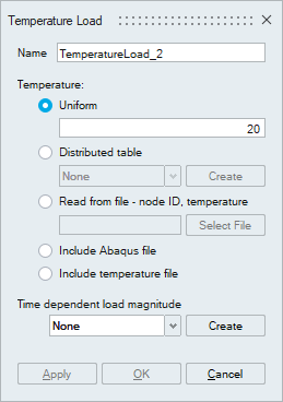
This tool is used to apply uniform (or) distributed temperature loads for thermal-stress analysis.
Description
- Distributed table option is used to apply a spatially varying
temperature load. The spatial temperature data has to be of the format
X,Y,Z,TemperatureValue.
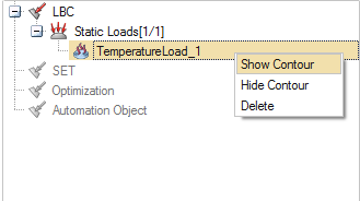
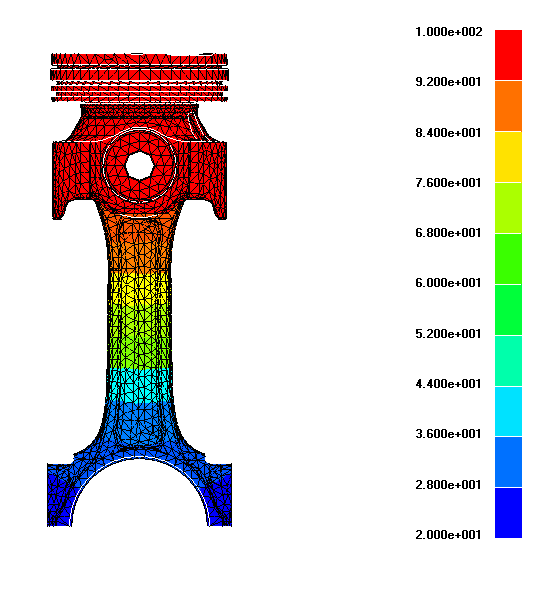
After applying the varying temperature load, the distribution can be visualized by contour plot. Right click the Temperature load in LBC browser and Select Show Contour option.
- Read from file - node ID,temperature option is used to specify a file containing temperature data in Node ID, Temperature format. This data will be directly included in the deck.(Supported only for Abaqus).
- Include Abaqus file option is used to specify a Abaqus *.fil or *.odb file generated during CFD (or) thermal analysis. This will be added as an include file in the Abaqus deck.
- Include temperature file option is used to specify a OptiStruct *.pch file generated during static / transient CFD (or) thermal analysis. This will be added as an include file in the OptiStruct deck. This option is available only for Nonlinear static analysis.
- Time dependent load magnitude option is supported for Non-linear
static solution & Static, Dynamic and Heat Transfer solution types.
Time-magnitude table can be given along with uniform, distribute table or
read from file options.
Cards supported for various solvers
| Solver | Supported Cards |
|---|---|
| OptiStruct / Nastran |
TEMP TEMPT (included transient temperature file) TABLED1, TLOAD1, DLOAD (if time-magnitude table is given) |
| Abaqus | *TEMPERATURE, bstep, binc, estep, einc, midside |
| Ansys | BFUNIF, BF |
| Permas | $DISLOADN |
| AdventureCluster | $Temperature |