
Create an Implicit Stochastic Lattice
Create a randomized strut lattice by defining points, edges between points, filters to remove certain points and/or edges, a method to thicken edges into struts, and outer body treatments such as combining the lattice with an outer body or shell.
A stochastic lattice arises from thickening a wireframe of the underlying structure, which is built up from points that are connected by edges. In Inspire Implicit Modeling, this wireframe structure is called a point-edge set. The general workflow for a stochastic lattice is as follows:
- Construct a set of (possibly random) points that are contained within a user-specified volume.
- Connect these points using one of the available methods to form edges.
- Filter the points and edges of the newly formed point-edge set to leave only the useful points and edges.
- Thicken the lattice according to your specifications for thickness (constant, variable-, or field-driven thickness).
- Apply outer body treatments to place a shell around the lattice, or join the lattice to a pre-existing outer body.

The rest of this topic describes these five steps in detail, explaining the different options for each.
-
Stochastic Lattice Point-Edge Set: Constructing Points
-
Click on the Stochastic Lattice icon in the Implicit Modeling
ribbon.
Tip: To find and open a tool, press Ctrl+F. For more information, see Find and Search for Tools.

-
Choose a setting from the point Generation Method dropdown
list.
Option Description Uniform Random Generates a user-defined number of points, using uniform distributions for each coordinate (x, y, and z). There are no guarantees or constraints on the emergent clustering or spacing of these points. - Select the Bounding Body that defines the volume in which the points will be contained. This can be done by clicking the body or selecting it from the Model Browser.
- Select whether the points should be contained
within the Body itself or the Bounds
of the axis-aligned bounding box of this body
(allowing some points to fall outside the body,
depending on the shape).


- Input a Seed for the random point generation; using the same seed will reliably reproduce the same set of points. Different seeds produce different point locations, which allows you to pick one that suits your requirements. This can be defined locally or controlled using a variable.
- Specify the Point Count, which is the number of points that will be created in the specified volume. This can be defined locally or controlled using a variable.
Minimum Separation Uses a proprietary algorithm to pack as many points into a volume as possible while maintaining a minimum conservative separation between each point. There are no guarantees on the number of points created, as this count emerges from the packing process. - Select the Bounding Body that defines the volume in which the points will be contained. This can be done by clicking the body or selecting it from the Model Browser.
- Select whether the points should be contained within the Body itself or the Bounds of the axis-aligned bounding box of this body (allowing some points to fall outside the body, depending on the shape).
- Input a Seed for the random point generation; using the same seed will reliably reproduce the same set of points. Different seeds produce different point locations, which allows you to pick one that suits your requirements. This can be defined locally or controlled using a variable.
- Specify the Minimum Spacing between points, which can be input locally as a constant, controlled using a variable, or defined using the field-drive icon, which means the minimum spacing can vary across the volume.
Import Can be used to import an externally generated set of points (stored in a .csv file) into Inspire. The .csv file for points should have three columns, each containing the x-, y-, and z-coordinates of the points. A header row, usually with the column titles, 'x', 'y,' and 'z', is required. Important: The units of this file should always be meters.
-
Click on the Stochastic Lattice icon in the Implicit Modeling
ribbon.
-
Stochastic Lattice Point-Edge Set: Constructing Edges
-
Choose a setting from the Generation Method
dropdown list.
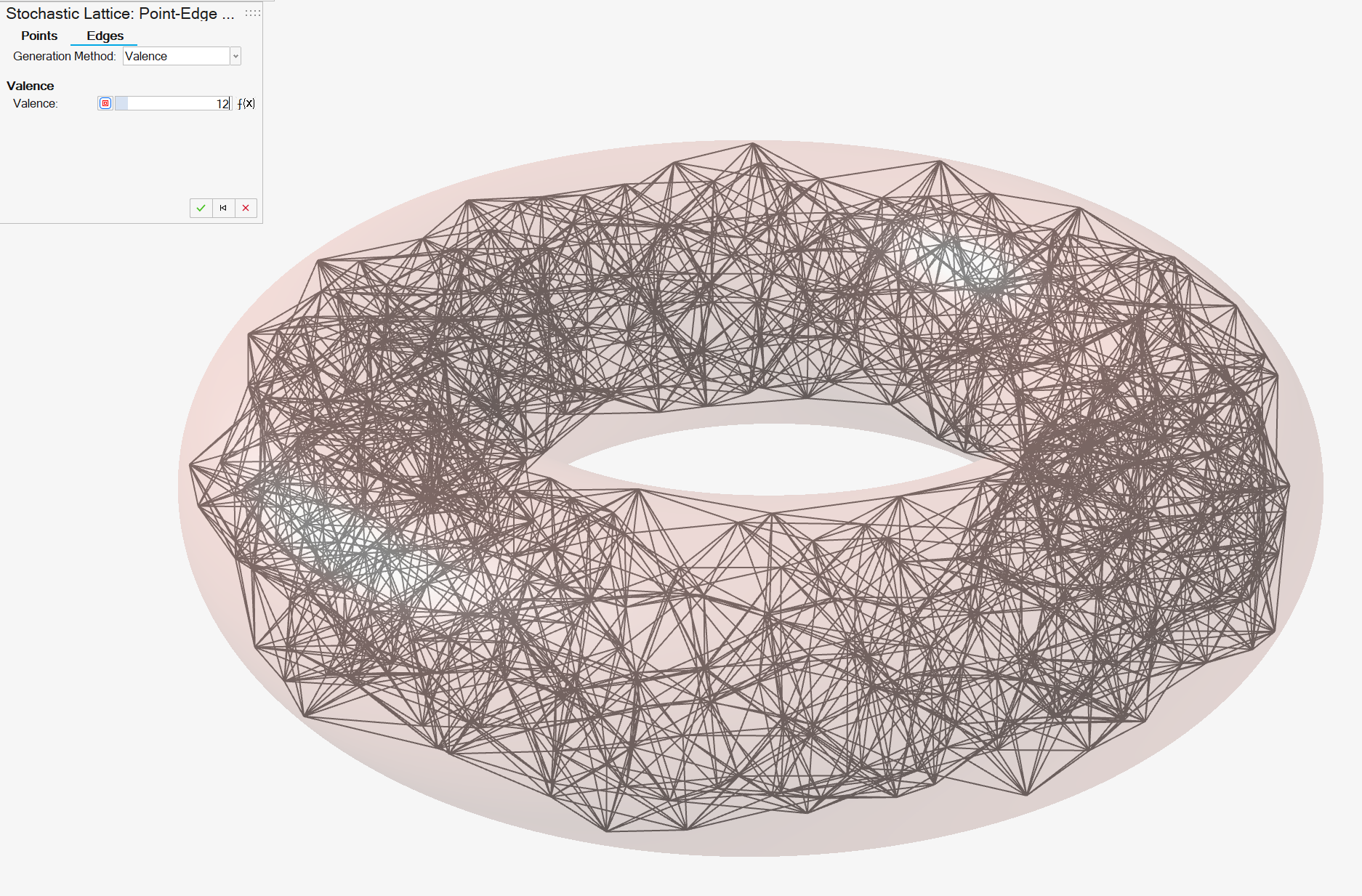
Option Description Valence Visits each point is turn and creates an edge between the point and its ‘k’ nearest neighbors. - The number of nearest neighbors it connects to is controlled using the Valence value, which can be set locally as a constant, controlled using a variable, or set using a field-driven property where ‘k’ varies in space according to the field value of the current point when interrogated against a user-specified field or implicit body. For example, if the current point is fed into a field and the field value at that location is 3.4, the valence for that point will be rounded to 3.0, which is the nearest integer value.
- The valence method does not offer any
guarantees over how many edges will be incident on
each point. This is because a point will connect
to its own nearest neighbors and other points may
connect to it if it is deemed a nearest neighbor
of those other points. Examples of
Valence = 4 and
Valence = 12 are shown
below.

Delaunay The Delaunay triangulation is created for all points in the point-edge set. There are no further options, as this triangulation is uniquely defined by the points in the set. In 3D, the Delaunay triangulation is better described as a Delaunay tetrahedralization. It has the property that the circumsphere of each of the four tetrahedral vertices does not contain any other point in the point-edge set. It should be noted that the Delaunay method will represent a volumetric mesh of the convex hull of the points. This means that long edges and edges that cross holes and other empty spaces are entirely possible. However, unwanted edges can be carefully filtered at a later stage of the workflow. 
Voronoi The points in the point-edge set are used as seeds to construct a 3D Voronoi diagram. A region called a Voronoi cell is constructed around each seed, and each region bounds all of the points that are closer to the associated seed than any other seed. Regions have planar faces, referred to as Voronoi faces. A Voronoi edge is formed where two or more Voronoi faces meet, and these edges are added to the point-edge set. An example of a Voronoi lattice is shown below. The Voronoi option may produce edges that travel externally with respect to the bounding body (first image, below). These can be removed later using suitable point-edge set filters as shown in the second image.


Import You can import a set of externally created edges stored in a .csv file. The .csv file for edges should have two columns, with a header row containing the titles Start and End to denote the start and end points for each edge. The entries for Start and End are integer references to the points in the aforementioned points .csv file. The first point has the index of 0 (i.e., 0-indexed). To create an edge between the first point and fourth point in the list of points, the edges file should contain an entry of 0 in the first column and 3 in the second column. When the points and edges have been created, the point-edge set is complete and you may click OK to accept the current configuration. This will progress the design to the next step, which takes place on the Stochastic Lattice guide panel. You should note that it is okay to have extra or unwanted points or edges at this stage, as these can be filtered later.
-
Choose a setting from the Generation Method
dropdown list.
-
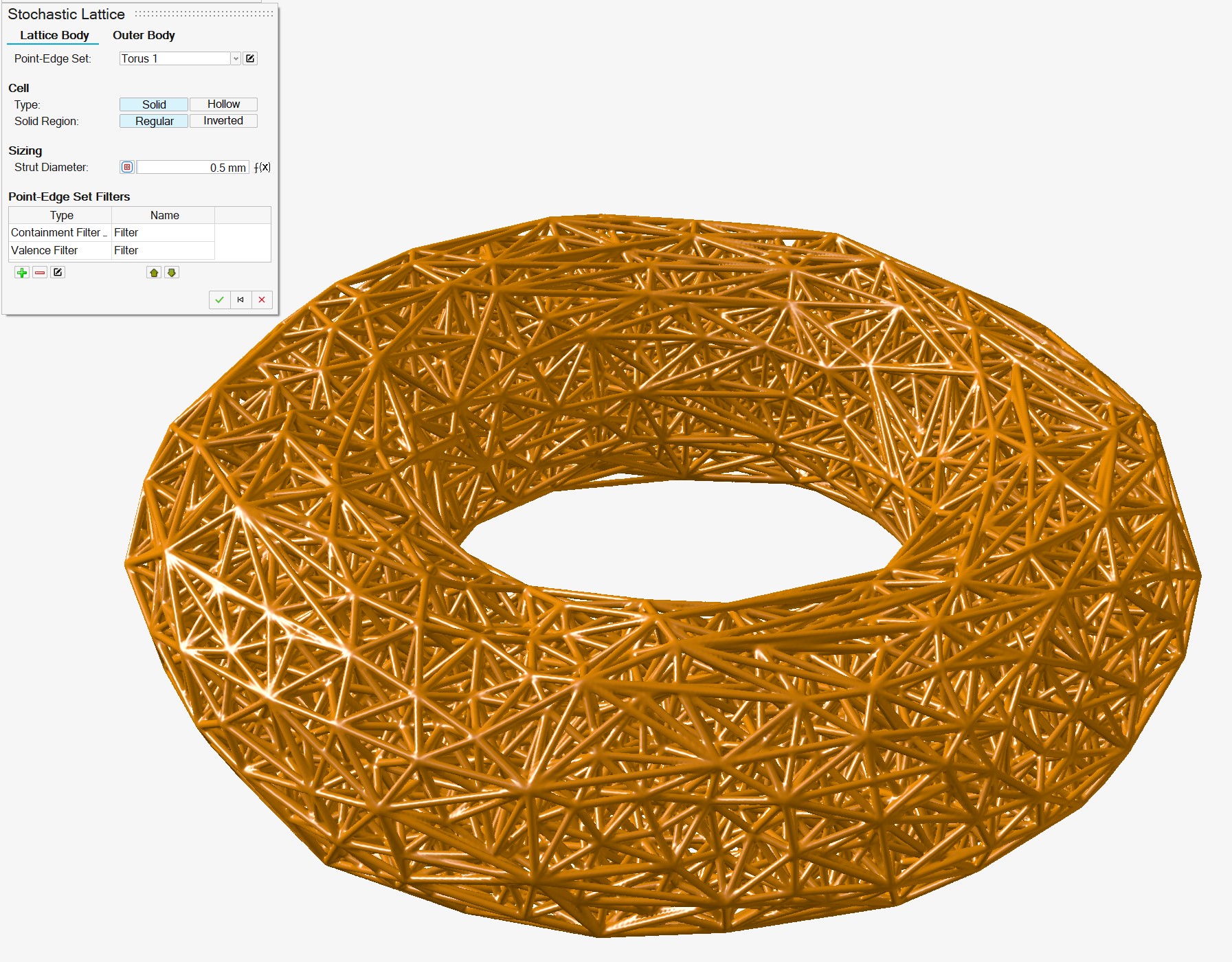
Stochastic Lattice: General Settings
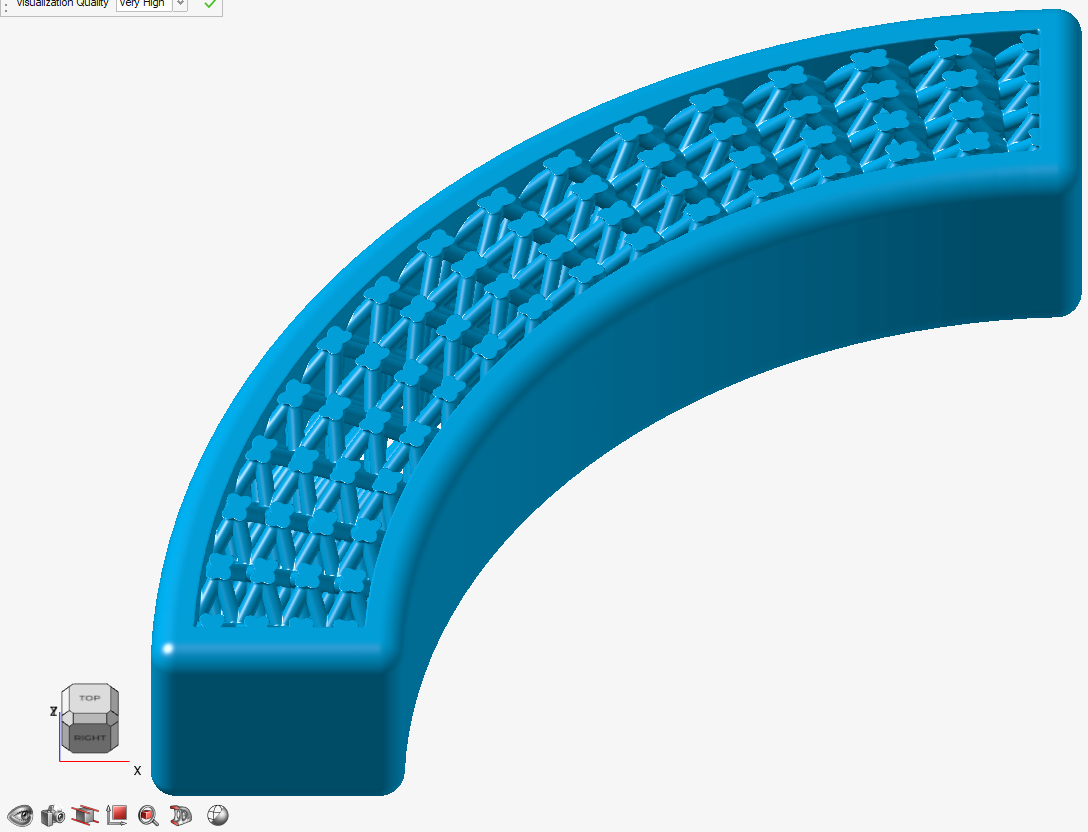
The Stochastic Lattice guide panel matures the wireframe model of the point-edge into an implicit model of the stochastic lattice by applying a default thickness. This model has the signed distance property. This means that any point in the field of this implicit body returns the signed distance to the closest point on the surface of the Stochastic Lattice. To clarify some terminology, an edge in the point-edge set becomes a strut in the stochastic lattice after it has been thickened.

- Choose a setting from the Point-Edge Set dropdown list to define the stochastic lattice structure. In most cases, this will be the point-edge set that has just been developed. However, there are options to choose a different set from the dropdown, make further edits, make a new set, or clear the selection, which will then require a new point-edge set to be created.
- In the Cell section, choose a
Type button to specify whether the struts
will be solid or hollow. Both types have a circular cross-section.
Therefore, a solid strut requires a single strut diameter, and hollow
struts require inner and outer diameter values.


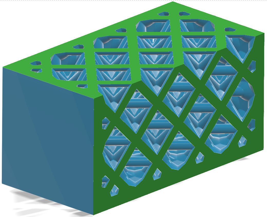
- Choose a Solid Region button to control whether
the stochastic lattice is defined by the struts themselves
(Regular) or by using the struts as tools to
cut material out of the axis aligned bounding box of the target body of
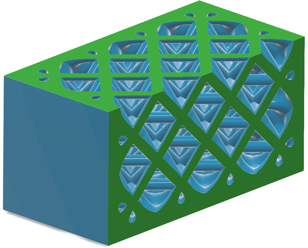
the Point-Edge set (Inverted). An example of the
Inverted case is shown below.
- Use the Sizing Options controls to specify the
inner and outer strut diameters. Strut diameters can be set locally as a
constant, controlled using a variable, or individually set a
field-driven properties, where the local radius at any point along any
strut is defined using a reference field or implicit body.Tip: The Strut Inner Diameter control is displayed only when Hollow is selected.
-
Stochastic Lattice: Point-Edge Set Filters
The methods for creating point-edge sets offer useful but limited flexibility over which points and edges are used in the final stochastic lattice. Much finer control is possible when filters are used. The following Stochastic Lattice guide panel shows an empty table of point edge set filters.
The buttons below the table can create, remove, edit, promote, and demote point-edge set filters.

When thinking about trimming a stochastic lattice to a shape, an important design consideration is whether to rely on a hard trim of a lattice using a Boolean Subtract operation, or whether to define the stochastic lattice so no trimming is necessary. In many cases, the latter is preferable, as it preserves the integrity of the point-edge set data structure. This can be useful when exporting the file to, for example, .3mf format (using the Beam Extension). Point-edge set filters provide facilities to make sure the lattice is nicely contained within a body, among other things.
-
Specify the filter rules.
Filters work by isolating a subset of points or edges from the overall point-edge set. In most cases, equality (=, ≠) or inequalities (<, >=, between, etc.) are used to express thresholds or ranges of values that determine whether a point or edge becomes part of the subset that will filtered (kept/removed).
- Filtering points
- Filtering by Bounding Body
identifies whether points are located inside a body/part
of interest. By default, points that fall inside (or on)
the bounding body are retained. Users can select CAD,
PolyNURBS, mesh, or implicit bodies for this filter.


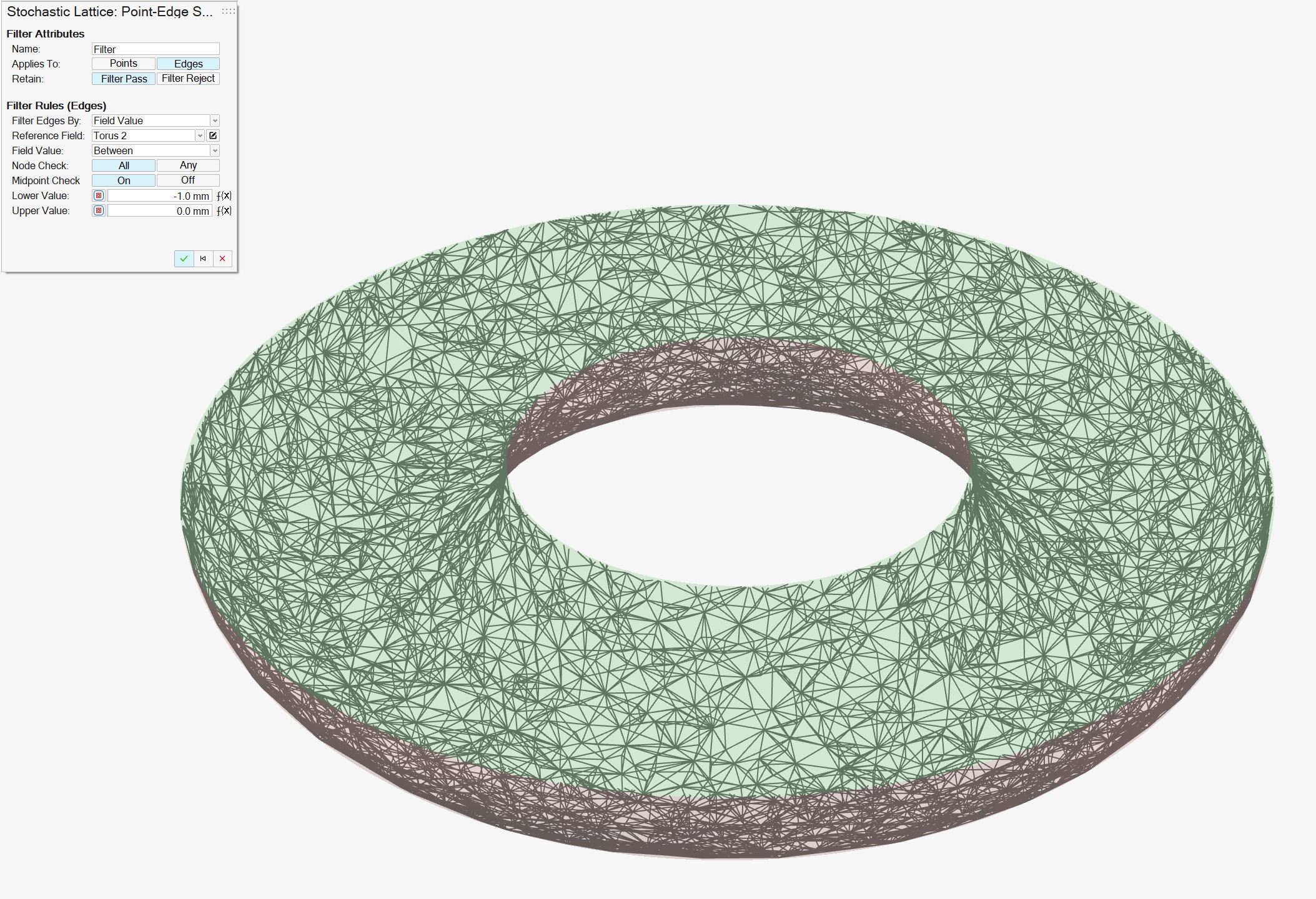
- Filtering by Field Value can be
used as query points within an existing field or
implicit body. The field value at the location of each
query point determines whether to keep or to remove the
point. In the following example, the field of the torus
is used to restrict the points in the point-edge set to
those lying between 0 mm and -3 mm (inside) from the
surface. The effect is a thin lattice wall in the shape
of a torus (shown in section for clarity).


- Filtering by Valence inspects the
number of edges that are incident on each point. Points
with too many or too few edges can be retained/removed
using this filter. The following images show a
Valence < 20 and
Valence < 16.
- Filtering by Bounding Body
identifies whether points are located inside a body/part
of interest. By default, points that fall inside (or on)
the bounding body are retained. Users can select CAD,
PolyNURBS, mesh, or implicit bodies for this filter.
- Filtering edges
-
Filtering by Bounding Body determines whether edges travel externally or internally with respect to the bounding body. When checking an edge, the two endpoints and an optional midpoint along the edge are checked. There are two options:
- All: Both endpoints and the optional midpoint fall inside the body.
- Any: Either endpoint or the optional midpoint fall inside of the body.
It is automatically assumed that the bounding body is the same body that was used to create the point-edge set. If this is not the case, you can select a different body using the Bounding Body selector.
To remove edges that travel externally with respect to the bounding body, use the Filter Pass result when Node Check is All and the Midpoint Check is On.Tip: Users should note that checking the endpoints and a midpoint does not guarantee that all externally traveling edges will be identified. However, it works well in most cases and computes quickly.


- Filtering by Length checks the
length of each edge to determine whether it is kept or
deleted. The following images show a point-edge set
before the length filter is applied, the same set with
edges limited to fall between 5 mm and 15 mm in length,
and the final struts. Note: No Bounding Body filters have been applied in these images. The external edges are simply removed as a result of their length.


- Filtering by Angle requires you
to select a reference geometry (a line, axis, planar
surface, or plane) from which to measure the angle. The
angle subtended by the edge and the reference geometry
is then used to determine whether edges are kept or
deleted. In the following example, the Z-plane is used
as a reference and any edges that have an angle of less
than 45 degrees to this plane are removed.


- Filtering by Field Value uses the
endpoints and an optional midpoint of each edge as query
points in a reference field. The field values for these
query points are then used to determine whether to keep
or delete the edge. As with Bounding
Body, there are two options:
- All: Both endpoints and the optional midpoint yield field values that meet the filter rules.
- Any: Either endpoint or
the optional midpoint yield field values that meet
the filter rule.
In the following example, the point-edge set has first been filtered by Bounding Body to remove edges that travel externally to the torus. Longer edges are then removed using an edge Length filter to restrict the set to beams <= 10 mm. Finally, the edges have been filtered by Field Value, using the torus's field as the reference field. Only beams where both endpoints and the optional midpoint have a field value between 0 mm and -1 mm are kept. This gives a thin shell of Delaunay-like lattice beams near to the surface as can be seen in the following section view.

- The Manufacturability filter is a compound filter that simultaneously considers the length and angle of each edge. As with the Angle filter, you select a reference geometry (line, axis, planar surface, or plane) to measure the angle of an edge. You also specify thresholds for length and angle that determine whether an edge is kept or deleted. This filter is designed to reflect that overhanging edges are more difficult to manufacture as they become longer.
-
- When you are happy with the filter, click OK to accept it. This will return you to the Stochastic Lattice guide panel, where you will see your new filter in the table.
- Filtering points
-
Specify the filter rules.
-
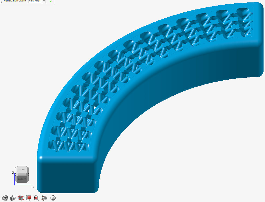
Select the Outer Body tab.
- Select a type of outer body.
- None: Don't create an outer body.
- Shell: Create an offset shell with an optional
trimming body.
Option Description Direction Select an offset direction for the shell. - Outward: Offset the shell outward from the lattice, increasing the size of the overall object.
- Inward: Offset the shell inward, consuming some of the lattice but maintaining the overall dimensions of the lattice.
- Both: Offset the shell both inward and outward.
Symmetry Symmetrically offset the shell inward and outward by the same distance. Outer Thickness Define the outward shell's offset thickness. Thickness can be entered directly, controlled with a variable, or controlled in each position in space using a field (field-driven design). 
Inner Thickness Define the inward shell's offset thickness. Thickness can be entered directly, controlled with a variable, or controlled in each position in space using a field (field-driven design). 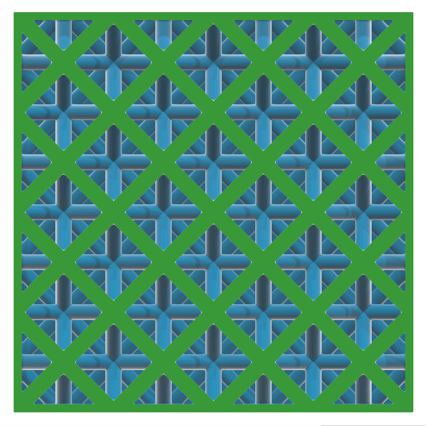
Trimming Body Select a body that's used to trim the shell. This can be used to trim areas of the shell, which is useful for fitting the lattice and its shell into a predefined volume, or when you want to expose some of the lattice so that it is not covered by a shell. In this example, a BRep body is chosen as the trimming body to expose some of the lattice. This image shows how the outward shell applied to the lattice overlaps with the trimming body.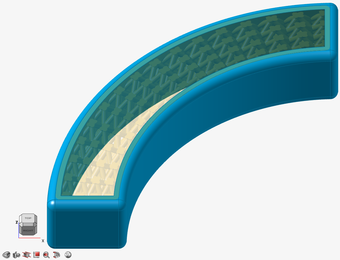 Once the trimming is applied, some of the outward shell is cut away, exposing the lattice wherever the shell protrudes beyond the confines of the trimming body.
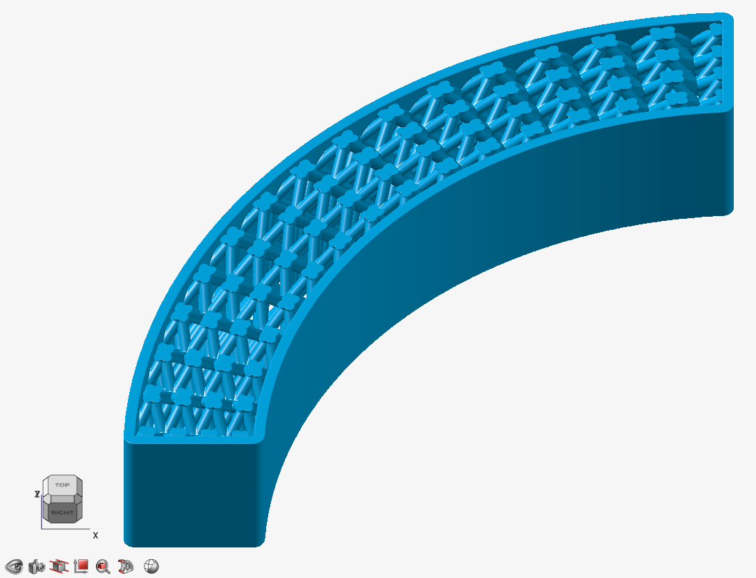
Transition Choose the type of transition between the outer body and lattice body. - Sharp: The lattice abruptly joins the surrounding shell.
- Fillet: The lattice
blends into the surrounding shell using a fillet.
If you selected this option, define the fillet
Radius.
- Chamfer: The lattice
blends into the surrounding shell using a chamfer.
If you selected this option, define the chamfer
Distance. For
Fillet, the distance is the
radius of the fillet and, for
Chamfer, the distance is
the setback of the chamfer. The distance can be
entered directly, controlled with a variable, or
controlled in each position in space using a field
(field-driven design).
- Combine: Combine the outer body with the lattice
body directly, without creating a shell that surrounds the lattice
Option Description Combine Body Select a body to combine the planar lattice with. This body should be close to or overlap the lattice. 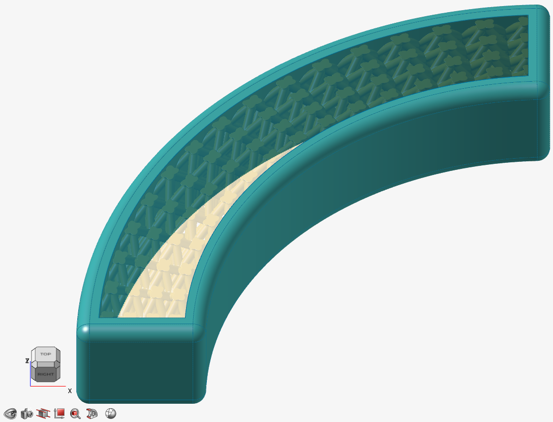
Transition Choose the type of transition between the outer body and lattice body. - Sharp: The lattice
abruptly joins the surrounding outer body.
- Fillet: The lattice
blends into the outer body using a fillet. If you
select this option, define the fillet
Radius.
- Chamfer: The lattice
blends into the outer body using a chamfer. If you
select this option, define the chamfer
Distance.

For Fillet, the distance is the radius of the fillet and, for Chamfer, the distance is the setback of the chamfer. You can directly enter the distance, controlled with a variable, or controlled in each position in space using a field (field-driven design).
- Sharp: The lattice
abruptly joins the surrounding outer body.