Results
Introduction
The following possibilities exist for postprocessing of results:
- inside SimLab
- Contour / Arrows / Isoline
- XY Plot
- Iso Surface
- Plot
- Node Path
- In the Flux environment by exporting to the solver and using all the functionalities available in the legacy Flux interface.
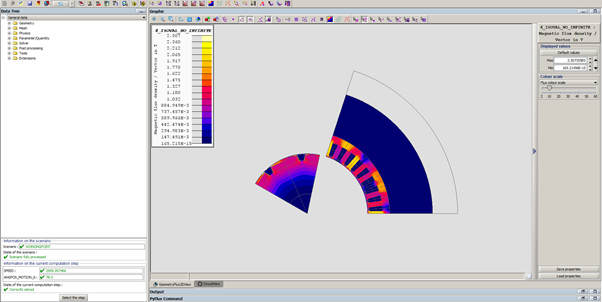
Contour / Arrows / Isoline
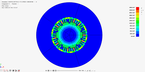
At the end of the solving, the contour results are displayed automatically. The contour or arrows and isoline options are visible on the graphical window top-left part.
Note that the full model (symmetry or periodicity) can be displayed by right click and selecting Show Full Model.
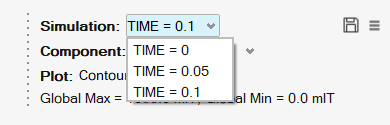
- The Simulation allows selecting the current step
(time or angular position or linear position)
To see the bodies animation, please use the animation tool bar:
 Note:
Note:The tool bar can be used in Transient Animation Mode, Modal Animation Mode and Linear Animation Mode:

- Transient Animation Mode is suitable for Magnetostatic solution, Transient Magnetic solution and AC Magnetic solution (complex quantity’s real part is displayed). The animation makes the time/position vary
- Modal Animation Mode can be used in AC Magnetic solution with or without Motion to display the complex vector results depending on the phase. The animation makes the phase vary
- Linear Animation Mode can be used in Magnetostatic solution without Motion
-
The possible Component for a 3D transient magnetic solution is the magnetic flux density B, the current density J and the Joule losses volume density dLossV if meshed coils are existing.
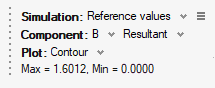
Note: To postprocess other quantities, please postprocess in Flux. - The Plot allows to choose between
contour or arrows:
- to display the color shade, choose Contour
- to display the arrows, choose Vector
- to display the isolines, choose Iso Line
For more details about the result panel, consult Result Panel.
For more details about the options of the scale, consult Result title and Legend bar.
For more details about the animation of the motion, consult Animate.
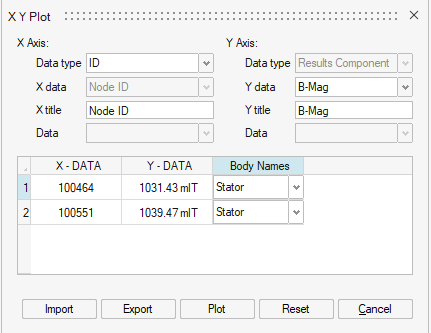
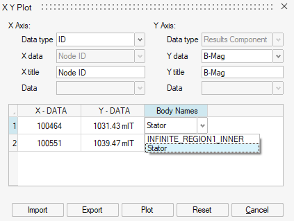
XY Plot

The XY Plot allows the user to do point computations.
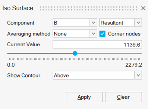
Iso Surface

The Iso Surface menu allows you to display for example the locations where B is greater or lower than a certain value, it allows to display the hot or cold spots.
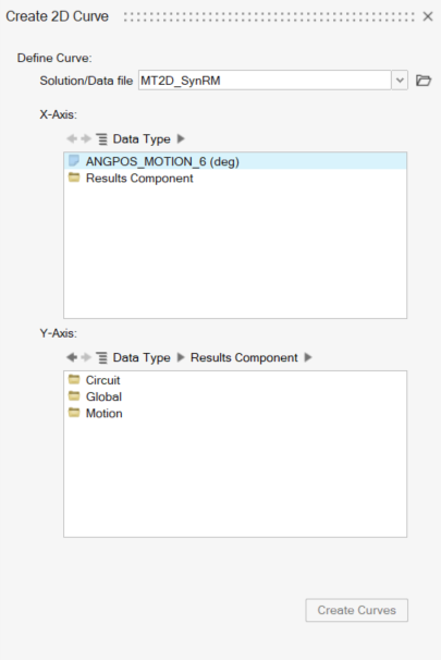
Plot

The Plot allows to post process global quantities chosen in the Result Request dialog box by the user.
- Circuit (current, voltage, ... of electrical components)
- Global (energy over the entire domain, ...)
- Motion (torque, force, ...)
Examples of Plots:
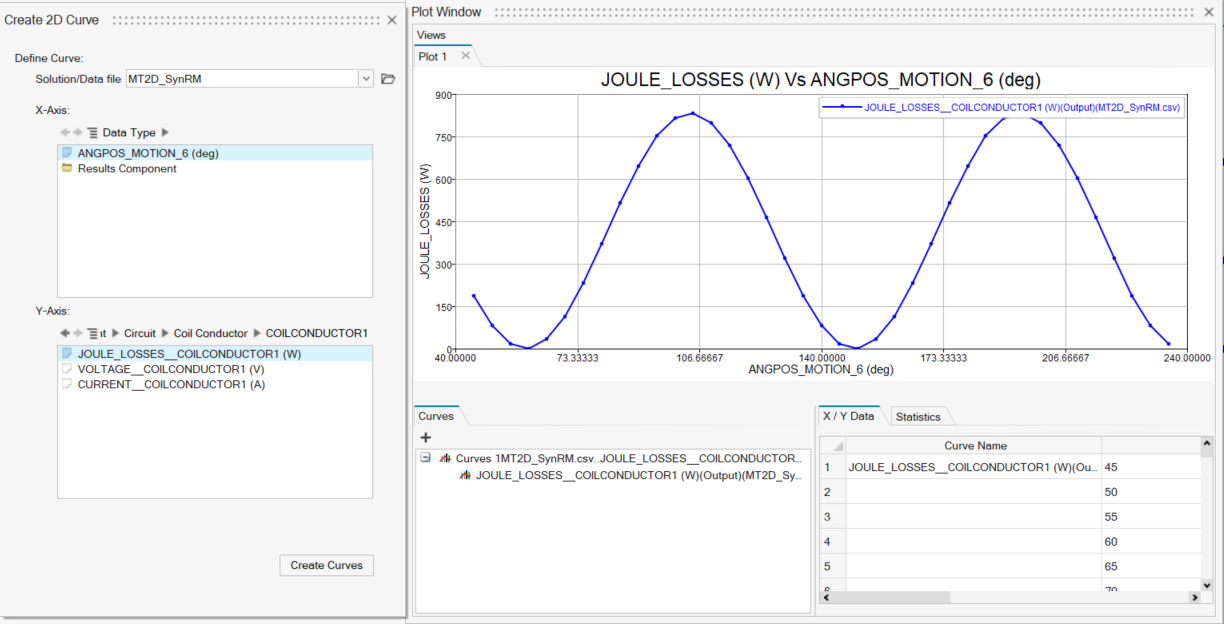
In the Circuit category:
The Joule losses of a coil conductor vs the angular position:
 Note: In 3D AC Magnetic solution, each quantity (Voltage / Current / …) is displayed for each component: Real, Imag, Module, Phase.
-
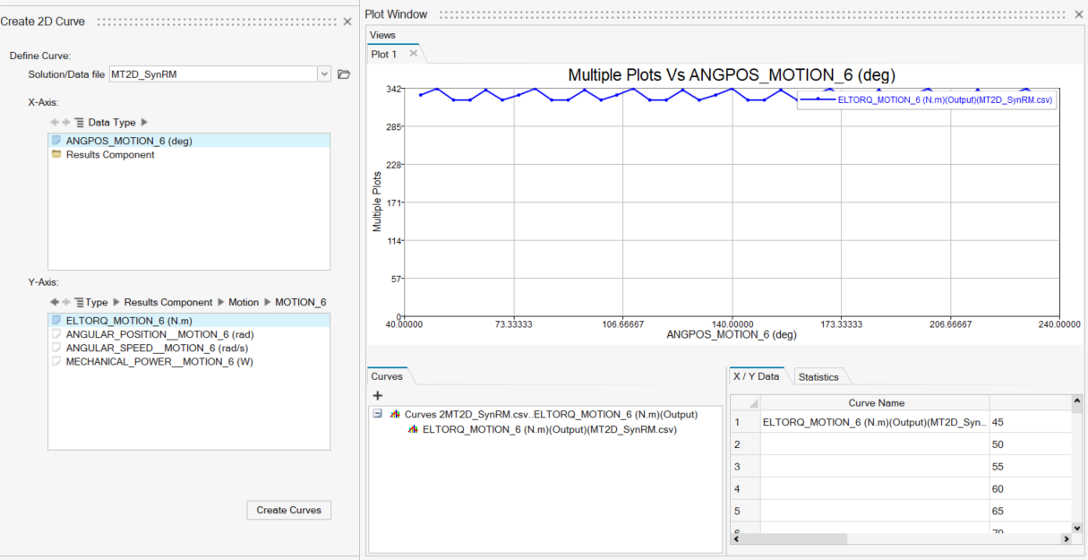
In the Motion category:
The electrical torque vs the angular position:
The created Plots are saved in the Solution Browser in Plots.
Node Path

Node Path allows to create the user defined paths and visualize the contour and vectors on the defined paths.
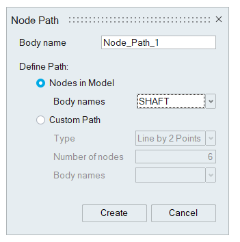
For more details about the node path, refer Node Path.
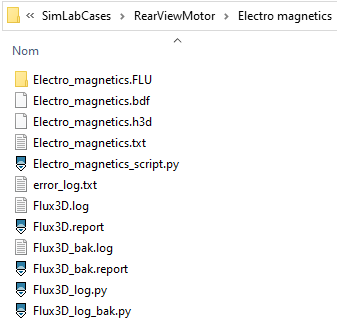
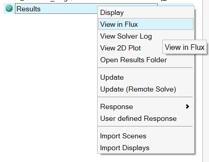
Postprocess in Flux
To access to Flux Postprocessing, in the Model Browser in the Assembly Tab, right click in Results and choose View in Flux.
Additionally to the project *.FLU other files are stored to be able to reproduce the full operations done (*.bdf, *.h3d, *.py) and log files to track a potential problem (*.log, *.report).