Result Panel
Introduction
The Results panel allows to visualize results by changing the options in the panel (load case, simulation, results component etc.)
To access the results panel, go to File | Preference | Results | Enable results panel option. This panel will vary based on the results model and component that are loaded.
Panel Options
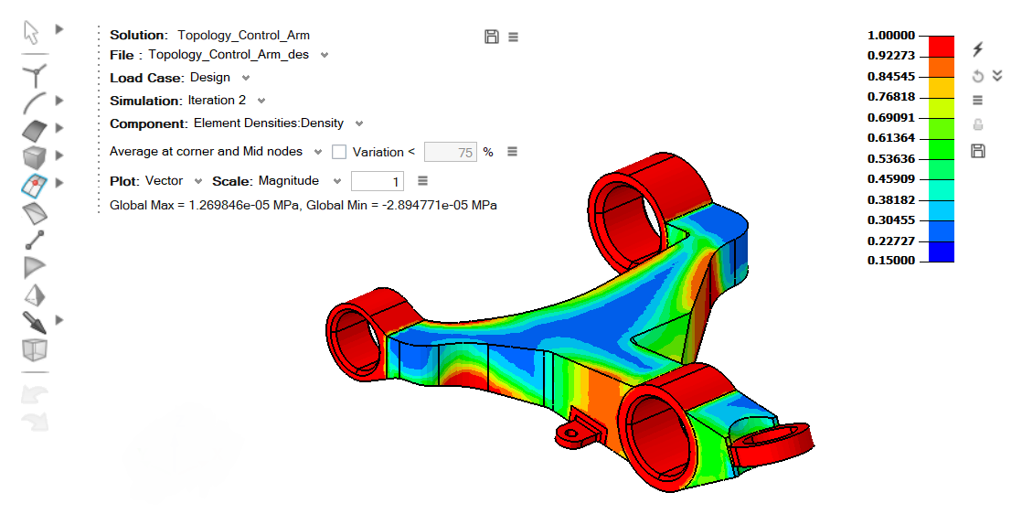
Solution
Shows the solution name of the displayed results.
File
Displays the imported results file name.
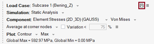
Load case
This option is used to select the various load cases in results file.
Simulation
This option is used to select different simulation available from selected load case.
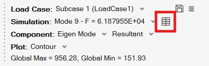
Modal Results Table
The Modal Results Table icon displays all computed normal modes and their natural frequencies in a table format.
This option is only available when the displayed results correspond to a Normal Model solution or a Normal Mode loadcase.
Selecting a mode in the table automatically displays the corresponding eigenvector (mode shape) in the graphics window as a contour plot.
Component
First menu will display various results types available in selected load cases and the second menu will shows the results component based on results types.
We will compute few result components in SimLab. Refer Computed Results for description.
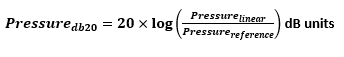
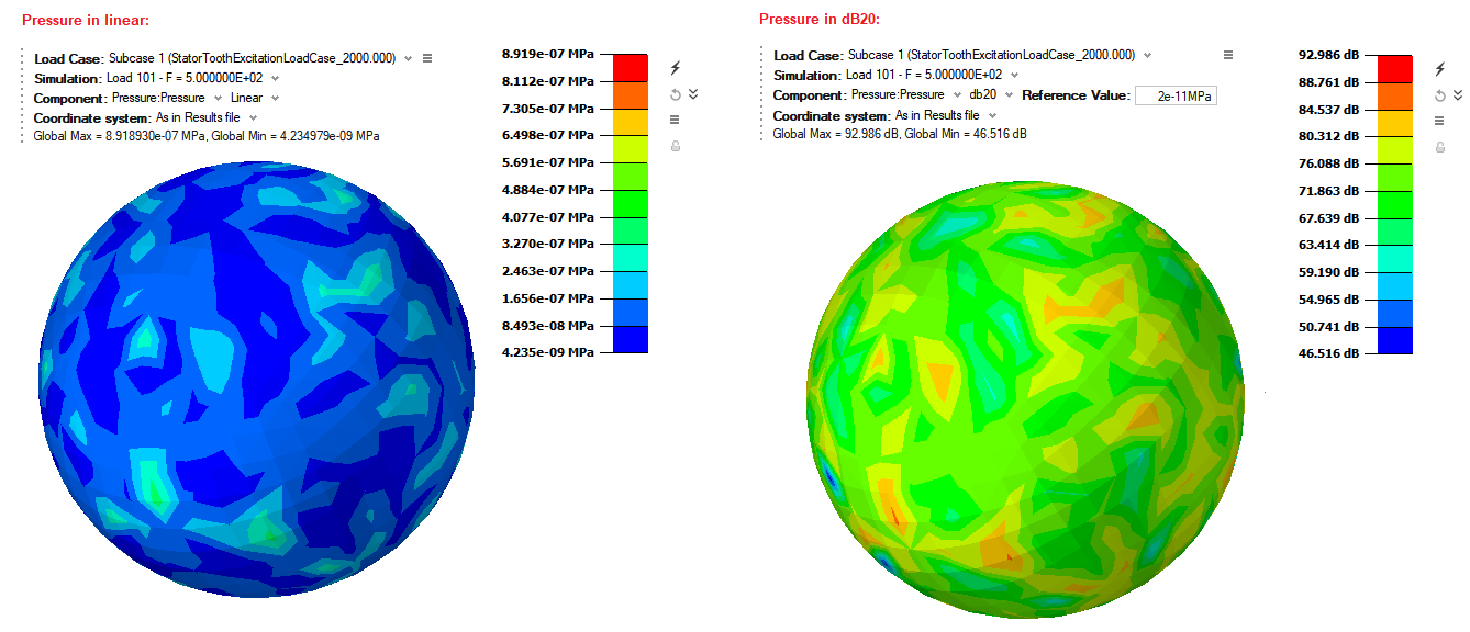
When the component is sound pressure, User can choose between linear or db20.
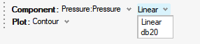
dB20 results computation formula:
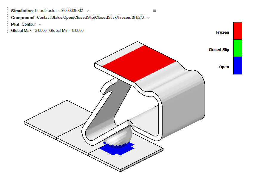
Supported to display the specific legend with status for the result components “Contact Status” and “Contact Coulomb Friction Status”.
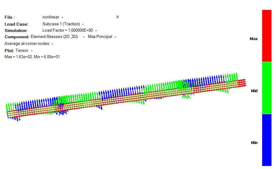
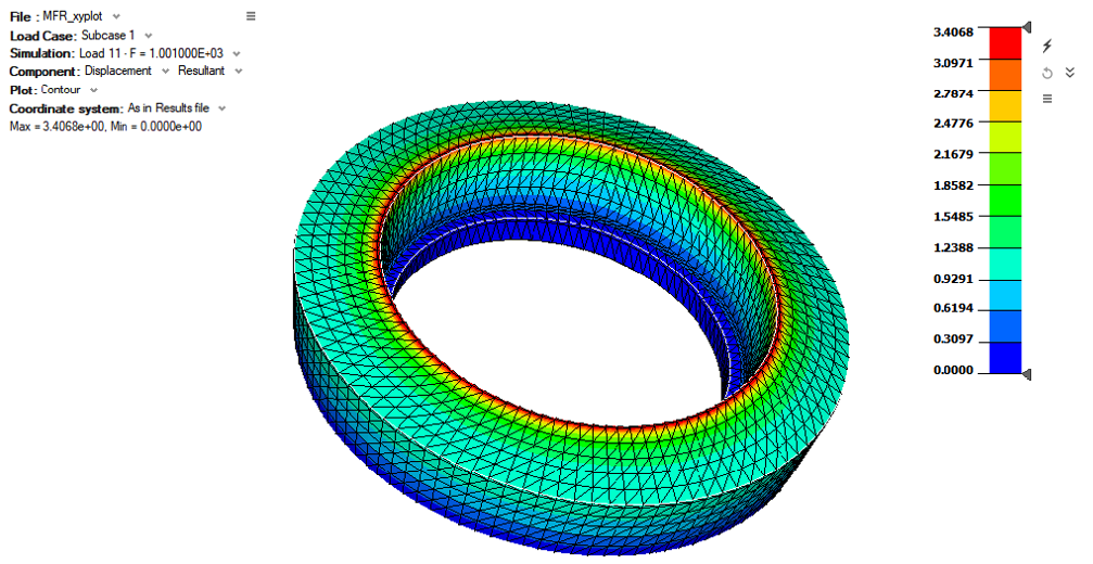
Plot options
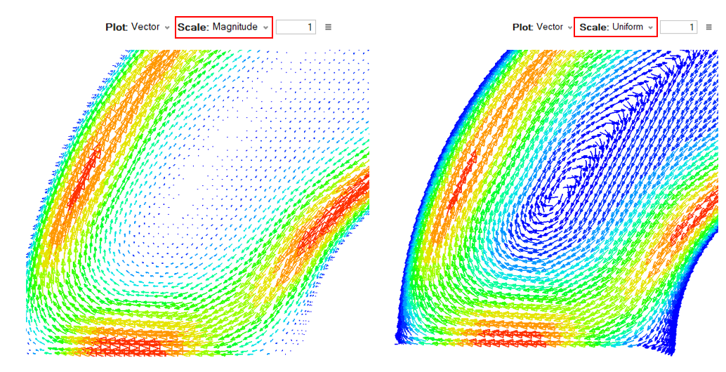
Option to change contour, vector, isoline and tensor plots.
- Vector plot supports both Magnitude and Uniform vector. Size of the vector is
editable
- For Optistruct results, vectors can be plotted by selecting multiple sub-components.
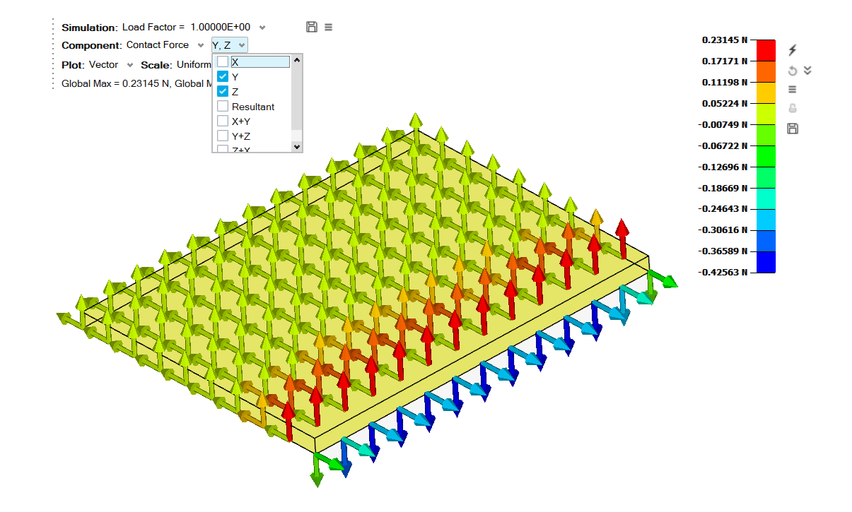
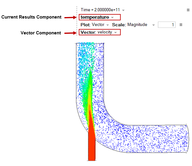
- For Acusolve and ElectroFlo results, vector scaling is based on the vector component
and vector coloring is based on the current results component. Mesh bodies are hidden
when vectors are activated.
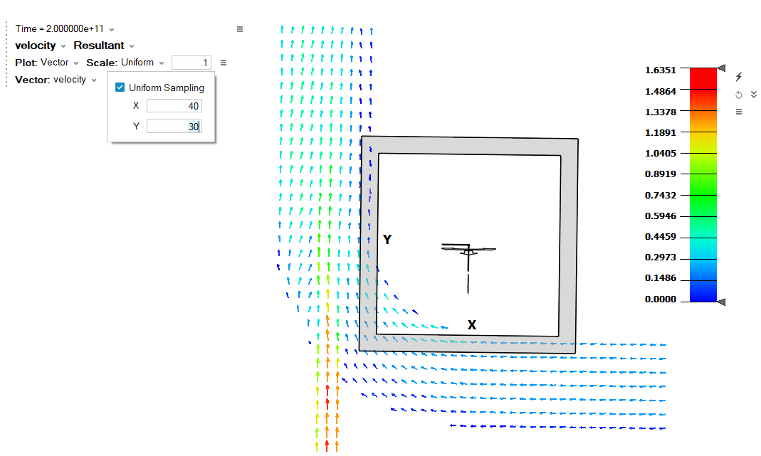
- Uniform sampling: Turn on this toggle to control the number of vectors
displayed along the cut section.
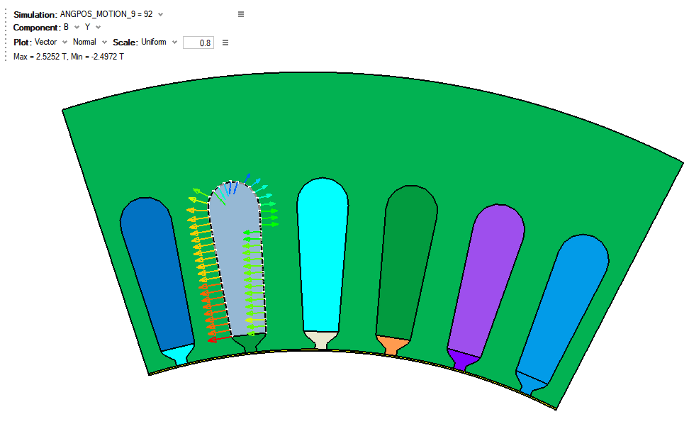
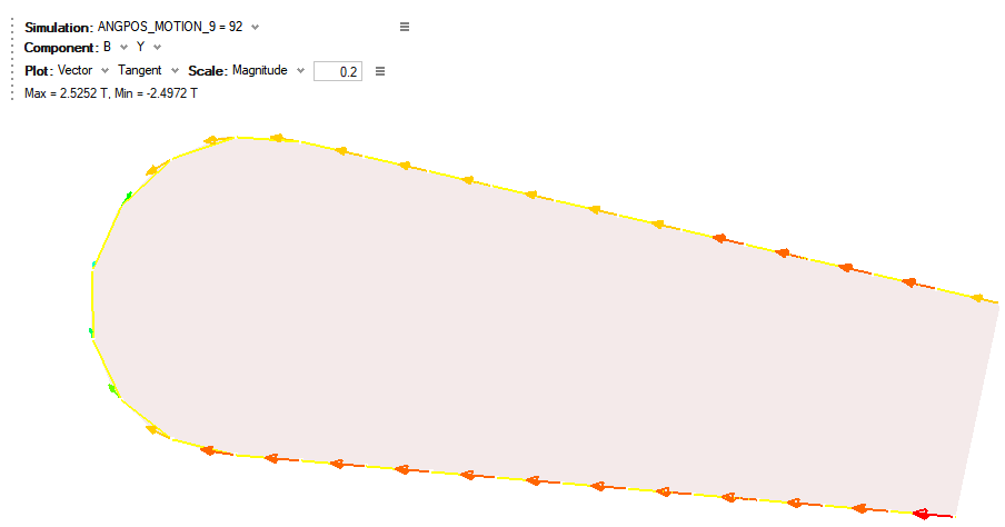
These are the options available to display the vectors along the result component, normal and tangential direction for the defined Node paths. Supported only for Flux results. Refer Node Path for how to create node paths.
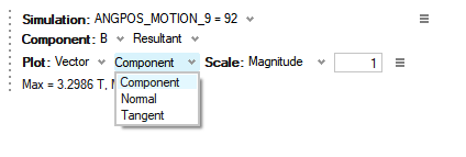
Vectors along Normal Direction:
Vectors along Tangential Direction:
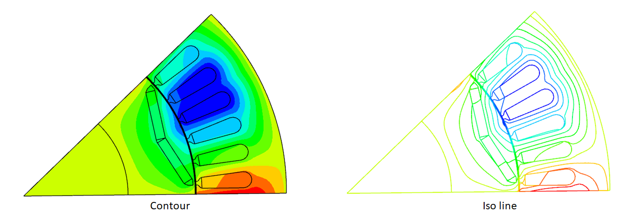
- Iso Line Visualization is supported for Flux results.
This option will be shown only in the following cases.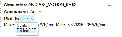
- 2D Models.
- Cut Layer display on 3D Model.
- Tensor plot is supported for principal components.
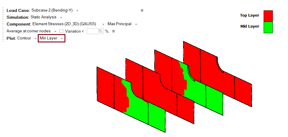
Layers
This option is to display a contour for a specified element layer when a layer definition is available for an element.
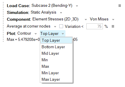
- Top Layer – Displays the contour for the top layer.
- Bottom Layer – Displays the contour for the bottom layer.
- Mid Layer – Displays the contour for the mid-layer.
- Min – Displays the minimum value among the layers for each entity.
- Max – Displays the maximum value among the layers for each entity.
- Min Layer – Identifies the layer that contributes to the minimum value for each entity. Displays the contour only for the shell elements.
- Max Layer – Identifies the layer that contributes to the maximum value for each entity. Displays the contour only for the shell elements.
Coordinate system
This option will display the coordinate systems available in the imported results file.
Averaging method
This option is used to select various averaging method for tensor results. We have few Averaging methods.
- Not Averaged
- Average at corner nodes
- Average at corner and mid nodes
- Maximum
- Minimum
- Advanced
- Difference
- Max of corner
- Min of corner
- Extreme of corner
- Volume Averaged
Click Here for more description.
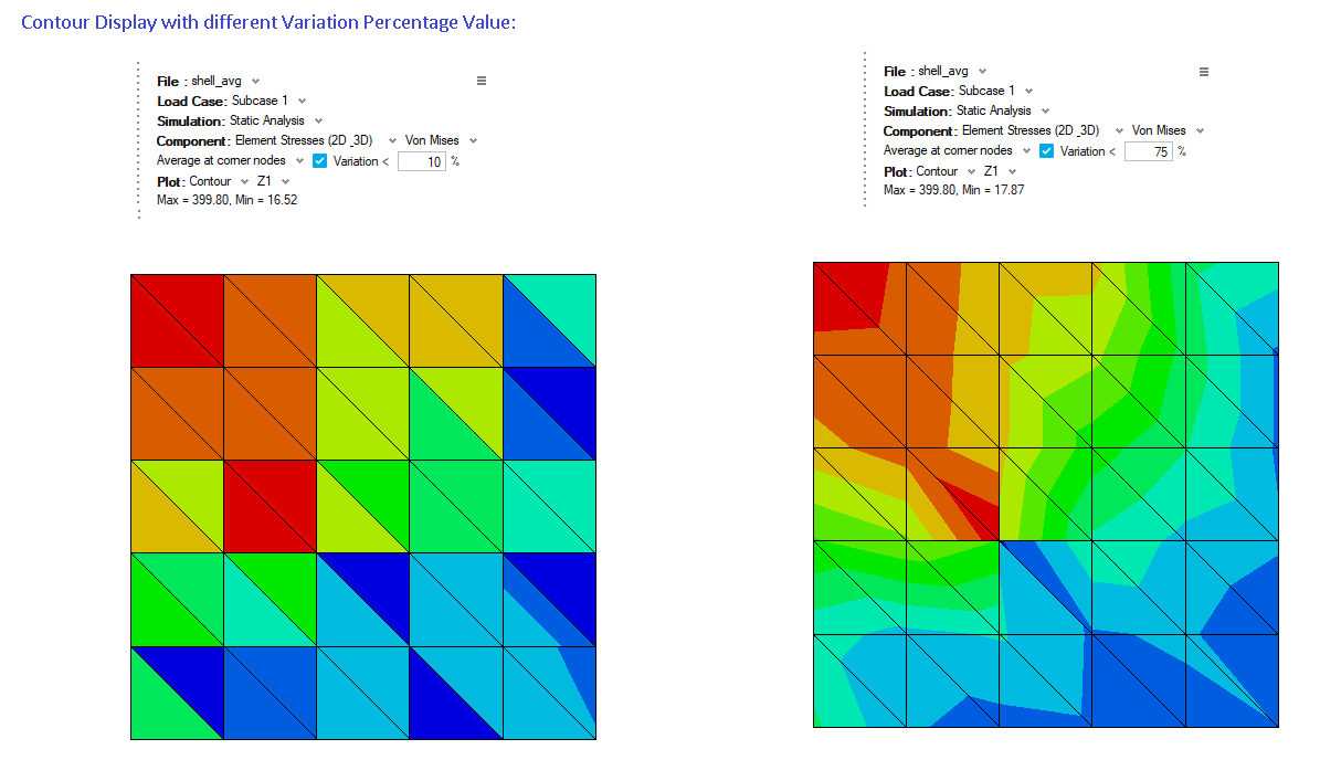
Variation Percentage Control
The variation is the relative difference at a node with respect to all nodes in the selected components.
The formula is described as follows:
Variation percentage at a node = (Difference at that node/Difference in all nodes from the selected components) x 100
For Example, the nodal variation (%) of tensor component xx at node 400 is calculated as follows:
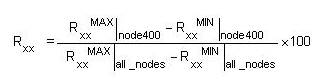
If Use variation (%) is off, the average results are calculated for all nodes. In this case, the results are node bound. If Use variation (%) is on, the average results are calculated for only some nodes, depending on the variation (%) you have defined. If the variation percentage is below the designated value at a node, nodal average at that node is calculated. Otherwise, corresponding element corner results at that node are used for contour plotting. 100% variation indicates all nodes will have average results; 0% variation indicates no nodes will have average results.
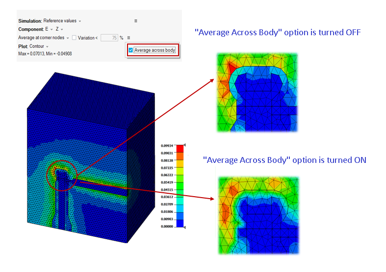
Average Across Body
Turn ON this toggle to enable the nodal averaging of results across the bodies. The contribution for a shared node will come from its associated bodies. This behaviour is applied for both "Average at Corner Nodes" and "Average at Corner and Mid Nodes" averaging methods.
Max and Min value
Displays current selected results component min and max value.
Complex Filters
The below options are available only when complex results are loaded.
- Mag - Magnitude of the complex result
- Phase - Phase of the complex number
- Real - Real part of the complex number
- Imaginary - Imaginary part of the complex number
- mag * cos (ωt- phase) - The response with varying angle or ωt (in degree).
- mag* cos (ωt + phase) - The response with varying angle or ωt (in degree).
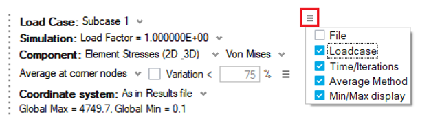
Show/Hide of Panel Options
To Show/Hide the panel controls, panel options available on the right side of the panel.
Reposition support
User can position the result title and legend bar anywhere in the graphics window.
Left mouse click on the title or legend bar to start the reposition. Then drag and drop in a convenient location.
By default, the results panel is on the top left of the graphics window.
For Acusolve and EFlow results, the panel is positioned on the top right of the graphics window.
Sub Results Panel
For EFlow solutions, supported to Create Sub Results Panel.
Save Display
Save Display option is used to save the current results panel settings and visualize multiple display of contour, vector and Isoline results.