Hydrodynamic Lubrication Model

The Hydrodynamic Lubrication contact model simulates the effect of short-range hydrodynamic forces on particles as though they were saturated in a fluid.

The model integrates the work of three studies (see References and Bibliography), resulting in a model that may be used for both Particle-Particle and Particle-Geometry contacts, with the assumption that the system is fully saturated, and no fluid free-surface is involved.

The model was developed to capture important macro-mechanical phenomena, such as strain-rate dependency and shear thickening, in dense granular suspensions, under shear and extensional flow. One of the key underlying assumptions for a dense suspension is that the particular volume fraction is high (φ > 0.45), which naturally leads to narrow gaps between the particles. This leads to a further assumption that the fluid flow in these gaps is laminar, meaning the model is most applicable in low-inertia systems and not in systems with turbulent fluid.

The model is a purely viscous model and is not applicable to static conditions. This model has been used to simulate shear and extensional flow in granular dense suspensions, though it may have a wider applicability.

Note: This model does not explicitly model the fluid, but its impact on particle behavior.

Calculating Particle-Particle Force and Torque

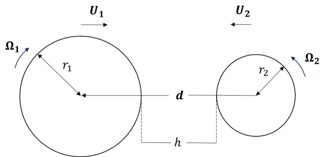
For particle-particle contacts, the model uses the theory as outlined in the work of Cheal & Ness (2018). In Figure 1, for two particles p₁ and p₂ with linear velocities U₁ and U₂, rotating at angular velocities Ω₁ and Ω₂, with center-center vector d, pointing from p₂ to p₁, with corresponding unit normal n=d/|d|, the force F and torque Γ acting on p₁ are defined as:

\begin{array}{l} \frac{F}{μ} = (X_{11}^{A} n \otimes n + Y_{11}^{A} (I - n \otimes n)) (U_{2} - U_{1}) + Y_{11}^{B} (Ω_{1} \times n) + Y_{21}^{B} (Ω_{2} \times n) \\ \frac{Γ}{μ} = Y_{11}^{B} (U_{2} - U_{1}) \times n - (I - n \otimes n) (Y_{11}^{C} Ω_{1} + Y_{12}^{C} Ω_{2}) \end{array}

where ⊗ is the outer product, μ is the viscosity of the fluid, and the remaining coefficients are defined as:

\begin{array}{l} X_{11}^{A} = 6 π r_{1} (\frac{2 β^{2}}{{(1 + β)}^{3}} \frac{1}{ξ} + \frac{β (1 + 7 β + β^{2})}{5 {(1 + β)}^{3}} \ln (\frac{1}{ξ})) \\ Y_{11}^{A} = 6 π r_{1} (\frac{4 β (2 + β + 2 β^{2})}{15 {(1 + β)}^{3}} l n (\frac{1}{ξ})) \\ Y_{11}^{B} = - 4 π r_{1}^{2} (\frac{β (4 + β)}{5 {(1 + β)}^{2}} l n (\frac{1}{ξ})) \\ Y_{21}^{B} = - 4 π r_{2}^{2} (\frac{β^{- 1} (4 + β^{- 1})}{5 {(1 + β^{- 1})}^{2}} \ln (\frac{1}{ξ})) \\ Y_{11}^{C} = 8 π r_{1}^{3} (\frac{2 β}{5 (1 + β)} l n (\frac{1}{ξ})) \\ Y_{12}^{C} = 8 π r_{1}^{3} (\frac{β}{10 (1 + β)} l n (\frac{1}{ξ})) \end{array}

where

ξ = \frac{2 h}{r_{1} + r_{2}}

h = |d| - (r_{1} + r_{2})

As mentioned in Cheal & Ness (2018) , the model is only intended to capture ‘short range contributions’. Therefore, interactions are only considered for an additional hydrodynamic force if they satisfy the following outer cutoff condition:

h \leq h_{o u t e r} r_{\min}

where r_min is the smallest of the two particle radii:

r_{\min} = \min (r_{1}, r_{2})

In addition to this condition, an additional inner cutoff condition is imposed so that the lubrication forces and torques are calculated down to a minimum separation distance of h_inner r_min.

For contacts that have h < h_inner r_min, the following is applied:

h = h_{i n n e r} r_{\min}

This means that hydrodynamic forces and torques are only calculated in the range:

h_{i n n e r} r_{\min} \leq h \leq h_{o u t e r} r_{\min}

But, these forces and torques are applied for all $h \leq h_{o u t e r} r_{\min}$

The default values are h_inner = 0.001 and h_inner = 0.05. This additional condition, and default values, are employed based on the approach of Cabiscol et al. (2021) , where the value of h_inner = 0.001 was selected to reflect the asphericity/roughness of the beads used in their experiments. This inner cutoff value should be adjusted according to the surface roughness of the material being modeled.

Figure 1. Schematic for two particles of radius r_1 and r_2, with linear velocities U_1 and U_2, rotating at Ω_1 and Ω_2, with center-center distance d, a distance h apart, approaching each other.

Calculate Particle-Geometry Force and Torque

The works of two sets of authors are used for resolving Particle-Geometry contacts - one for calculating the normal force component (Goddard et al. (2020)) and the other for calculating the tangential force and torque components (O'Neil & Stewartson (1967)). All Particle-Geometry contact models follow the same cutoff implementation as the Particle-Particle model, using the approach of Cheal & Ness (2018) .

Normal Force

There are two possible approaches for the calculation of the normal force, both outlined in Goddard et al. (2020). One follows an analytical approach, henceforth referred to as Goddard_log, and the other follows a numerical approach, henceforth referred to as Goddard_sum.

For Goddard_log, following the approach of Goddard et al. (2020), for a particle of radius r₁ approaching a Geometry element with an assumed radius r₂, that is very large, the ratio of their radii is defined as:

β = \frac{r_{2}}{r_{1}}

The gap between the particle and Geometry is termed ε, which is non-dimensionalized by the particle radius as shown in the following figure.

The non-dimensional normal force on the particle as it approaches the Geometry in the normal direction is then defined as:

F_{n}^{*} = \frac{(2 β^{2})}{ε {(1 + β)}^{2}} - \frac{2 β (1 + 7 β + β^{2})}{5 {(1 + β)}^{3}} l n (ε) + K_{2} (β)

where higher order terms have been ignored. K₂ has been calculated as described in equation (B21) in the Appendix of Goddard et al in References and Bibliography. As the calculation is complex, steps for calculation are omitted here. See the original paper for its calculation.

Considering that the radius of the Geometry element is assumed to be quite large, the resulting force experienced by the particle after re-dimensionalization with the typical drag scale 6πμU_r1 is defined as:

F_{n} = 6 π μ U r_{1} (\frac{2}{ε} - \frac{2}{5} \ln (ε) + K_{2})

where 2U is the relative approach velocity between the particle and Geometry and μ is the fluid viscosity.

Figure 2. Schematic of a Particle of radius r1 traveling at a velocity U normally towards a Geometry of radius r2, which is moving at a velocity U towards the particle, with a non-dimensional separation distance of ε.

Using the definitions of ε, r₁, r₂, U, and μ as mentioned above, for the approach of Goddard_sum, also outlined in Goddard et al. (2020), the dimensional normal force on the particle as it approaches the Geometry in the normal direction is calculated by:

F_{n} = - \sqrt{2} c π μ u \sum_{n = 1}^{\infty} (2 n + 1) (a_{n} + b_{n} + c_{n} + d_{n})

where c > 0 is a geometrical constant, defined as follows, and a_n, b_n, c_n, d_n (η) are series coefficients, dependent upon η, defined as follows. The complete definition of these series coefficients are omitted for brevity though they are defined in Goddard et al. (2020). An equal and opposing force is applied to the Geometry.

The approach of Goddard_sum uses spherical bipolar coordinates (η, ξ, θ) to represent both particle and Geometry as constant values of η, which conveniently represents two non-intersecting coaxial spheres, with centers in the Cartesian plane at (0, c coth(η)), and radii c | csch(η)|. Designating the distance from the center to center of element i to the origin O (taken to be the contact point) by d_i and its radius to be r_i, the spherical bipolar ordinates that define the particle (element 1) and Geometry (element 2) are as follows:

\cosh (η 1) = \frac{d_{1}}{r_{1}}, \cosh (η 2) = \frac{d_{2}}{r 2}

Figure 3 provides a visual representation of this definition, which is not commonly used in DEM. For more information about the approach, see Goddard et al. (2020).

Figure 3. Schematic of a particle of radius r1 traveling at a velocity U normally towards a Geometry of radius r2, which is moving at a velocity U towards the particle, with center-center distance d, a dimensional separation distance of h and with β=r1/r2. Note that the Geometry radius is much larger than that depicted in the figure.

Tangential Force and Torque

Following the approach of O’Neil & Stewartson (1967), consider the scenario of a particle of radius r moving parallel to a Geometry. The non-dimensional gap between the particle and Geometry is termed ε, as outlined previously and shown in the following figure.

The tangential force exerted on the particle is then defined as:

F_{t} = 6 π μ U r f

where

f = (\frac{8}{15} + \frac{64}{375} ε) \ln (\frac{2}{ε}) + 0.58461

and the higher order terms in ε have been ignored. An equal and opposite force is applied to the Geometry.

The torque applied is defined as:

T = 8 π μ U r^{2} τ_{i}

where, for the particle:

τ_{i} = (\frac{1}{10} + \frac{43}{250} ε) \ln (\frac{2}{ε}) - 0.26277

and for the Geometry:

τ_{i} = (\frac{1}{10} + \frac{43}{250} ε) \ln (\frac{2}{ε}) - 0.26221

The higher order terms in ε have been ignored.

Figure 4. Schematic of a particle of radius r traveling at a velocity U parallel to a Geometry surface, with a non-dimensional separation distance of ε.

Cutoffs

The inner and outer cutoffs explained previously for Particle-Particle contacts (and in Cabiscol et al. (2021) ) are also utilized for Particle-Geometry interactions, which means that the forces and torques outlined as follows are only ever calculated in the range:

h_{i n n e r} r_{\min} \leq h \leq h_{o u t e r} r_{\min}

but are applied for all $h \leq h_{o u t e r} r_{\min}$ where h_inner, h_outer, and r_min are as described previously.

Using the Hydrodynamic Lubrication Model

To use the Hydrodynamic Lubrication contact model, you must first add it to the Physics of a given EDEM simulation and then configure as required.

The model will run without a contact radius specified for the particles, but to capture the full range of forces, you must specify a contact radius that will cover separations up to the specified outer cutoff . This means that the contact radius should be at least half of the outer cutoff distance on top of the physical radius. For example, with the default outer cutoff defined at 0.05 r_min , the contact radius should be at least 1.025 r_min , so that when two contact radii just touch, the center-to-center distance of the particles is 2.05 r_min. and hence the gap between the particles is 0.05 r_min.

Also, while you can enable the model while using polyhedral particles which currently do not have a contact radius, the full range of forces will not be applied correctly. You must proceed with caution when you want to use polyhedral particles with the model.

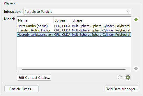
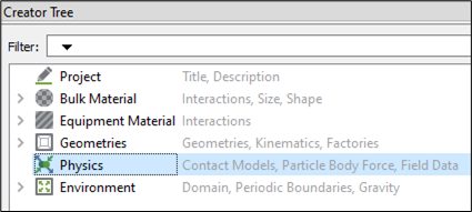
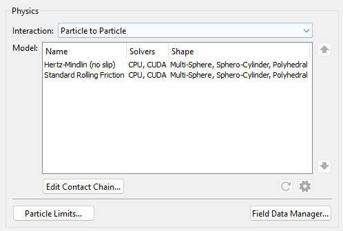
In the Creator Tree, select Physics.
Select Particle to Particle and/or Particle to Geometry from the Interaction dropdown list.
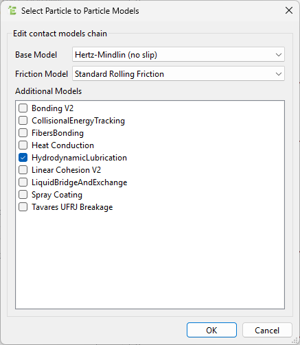
Click Edit Contact Chain at the lower section of the Physics panel.
Under Plug-in Models, select the HydrodynamicLubrication checkbox.
Click OK.
The plug-in is displayed in the Model panel.
Select the plug-in and click the icon in the lower-right section of the Physics panel to configure it.
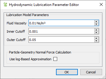
In the Hydrodynamic Lubrication Model Parameter Editor dialog box, specify values for Fluid Viscosity, Inner Cutoff, and Outer Cutoff.

The Inner and Outer Cutoff values correspond to the non-dimensional values (by particle radius) between which the additional forces and torques are calculated. (The inner cutoff value should be adjusted according to the surface roughness of the material being modeled. (For more information about specifying cutoff values, see Cabiscol et al. (2021)).

Note: Because one of the assumptions for the theory is that the particles are fully saturated with fluid, these values are applied to all particles in the simulation, rather than by type or interaction. As noted by Cabiscol et al, due to the omission of long-range fluid effects in the model, using the real fluid viscosity may not yield the same behavior as in the real-world. It has the same units and plays the same role as the real fluid viscosity, but it is recommended to perform a calibration on the fluid viscosity (as well as inner and outer cutoff values) to obtain the correct material behavior.
Select the additional checkbox for the Particle-Geometry contact model to allow selecting the Goddard_log implementation for normal force.
The most recommended default implementation is that of Goddard_sum. You can select Goddard_log only if a simulation is already using the Hydrodynamic Lubrication model from EDEM v 2023.1, which only had the Goddard_log implementation, and to ensure consistency.
After specifying the values, click OK.

Post Processing

Lubrication forces and torques are directly added to the particle characteristics Total Force and Total Torque. As a result, they are difficult to analyze separately from other contact forces and torques.