Fibers Bonding Model

The Fibers Bonding Model keeps particles bonded in order to simulate long structures like fibers, stems, branches, or strings.

The model is designed to work with Sphero-Cylinders. You must create a Meta-Particle using Sphero-Cylinders which overlap physically (no contact radius to be used). The particles in the Meta-Particle can be bonded end-to-end or at oblique angles.

The bond emulates the flexibility of the adjacent particles, from their center to the contact point, originating from the theory of beams. The model applies a bonding force and a bonding torque to both particles according to a set of stiffnesses, which can be decomposed into one axial stiffness, two shear stiffnesses, one torsional stiffness, and two bending stiffnesses. Currently, the two shear stiffnesses and the two bending stiffnesses are also equal.

Calculating Particle-Particle Force

If you add the interaction between two bulk materials to the model configuration, two particles from those two materials may be bonded. For a bond to form, the bond creation time (which is a particle custom property) of both particles must be the same, and contact at the bond creation time. By default, factories in EDEM are configured to set the bond creation time to the particle creation time such that the particles within a Meta-Particle can be bonded when the Meta-Particles are created. The contact point detected by EDEM will not be used by the model at any time except during the bond creation. The force exerted by the bond on particle 1 is defined as:

F_{1} = - K_{1} {(K_{1} + K_{2})}^{- 1} K_{2} (x_{1} - x_{2})

where

K_{1} = R_{1}^{T} K_{1}^{'} R_{1}

K_{2} = R_{2}^{T} K_{2}^{'} R_{2}

are the displacement-related stiffnesses brought by particle 1 and particle 2 to the bond in global coordinates. K^'₁and K^'₂ are defined as:

K_{1}^{'} = α_{d i s p} (\begin{matrix} \frac{E_{1} A_{1}}{d_{1}} & 0 & 0 \\ 0 & \frac{G_{1} A_{1}}{d_{1}} & 0 \\ 0 & 0 & \frac{G_{1} A_{1}}{d_{1}} \end{matrix})

K_{2}^{'} = α_{d i s p} (\begin{matrix} \frac{E_{2} A_{2}}{d_{2}} & 0 & 0 \\ 0 & \frac{G_{2} A_{2}}{d_{2}} & 0 \\ 0 & 0 & \frac{G_{2} A_{2}}{d_{2}} \end{matrix})

Representing the same stiffness matrices in local coordinates to both sides of the bond, where R₁ and R₂ are the rotation matrices between local and global coordinates at both sides of the bond, E is the Young's modulus, G is the Shear modulus, A is the cross-sectional area, d₁ and d₂ are the distances between the particle centers and the contact point, and α_disp is a coefficient to increase or decrease the stiffness called the Force Stiffness Scaling Factor.

The force exerted by the bond on particle 2 is defined as:

F_{2} = - F_{1}

Calculating Particle-Particle Torque

The torque exerted by the bond on particle 1 is defined as:

T_{1} ​ = R_{1}^{T} ​ T_{1}^{'} ​ R_{1}

The torque exerted by the bond on particle 2 is defined as:

T_{2} ​ = R_{2}^{T} ​ T_{2}^{'} ​ R_{2}

Both torques are the expression in global coordinates of their counterparts in local coordinates defined as:

T_{1}^{'} = Q_{1}^{'} [\begin{array}{l} θ_{t w i s t, 1} \\ θ_{b e n d, 1 a} \\ θ_{b e n d, 1 b} \end{array}]

T_{2}^{'} = Q_{2}^{'} [\begin{array}{l} θ_{t w i s t, 2} \\ θ_{b e n d, 2 a} \\ θ_{b e n d, 2 b} \end{array}]

where θ_twist,1 is the twist angle of particle 1 from its center to the bond (analogous for particle 2), and θ_bend,1a and θ_bend,1b are the bending angles of particle 1 from its center to the bond, around two perpendicular axes (a and b) to the bond orientation at the side pointing towards particle 1 (analogous for particle 2). The torque stiffness matrices in local coordinates are defined as:

Q_{1}^{'} = α_{r o t} (\begin{matrix} \frac{G_{1} J_{1}}{d_{1}} & 0 & 0 \\ 0 & \frac{E_{1} I_{1}}{d_{1}} & 0 \\ 0 & 0 & \frac{E_{1} I_{1}}{d_{1}} \end{matrix})

Q_{2}^{'} = α_{r o t} (\begin{matrix} \frac{G_{2} J_{2}}{d_{2}} & 0 & 0 \\ 0 & \frac{E_{2} I_{2}}{d_{2}} & 0 \\ 0 & 0 & \frac{E_{2} I_{2}}{d_{2}} \end{matrix})

where I_i are the moments of inertia of the cross-section of the respective particle, J are the polar moments of inertia of the same section, and α_rot is a coefficient to increase or decrease the torque stiffness called the Torque Stiffness Scaling Factor.

In the general case, T₁ and T₂ are not equal if we consider that the bond keeps the same, constant orientation. As a result, the model recomputes the orientation of the bond at every Time Step to ensure that $T_{1} = - T_{2}$

Damping

Following the concept of Rayleigh damping from the Finite Element Method, this model damps the relative velocities and relative angular velocities of the two particles in contact. The model, however, does not damp the possible high velocities or angular velocities of the particles themselves. This means that the model only takes the stiffness matrix from the damping matrix of Rayleigh damping, ignoring the mass matrix (which would introduce a less realistic damping).

The damping forces are defined as:

F_{d, 1} = - α_{d a m p ​} K_{1} {(K_{1} + K_{2})}^{- 1} K_{2} (v_{1} - v_{2})

F_{d, 2} = - F_{d, 1}

where v₁ and v₂ are the velocity vectors of both particles at the contact point.

Similarly, the damping torques are defined as:

T_{d, 1} = - α_{d a m p} ​ ​ Q_{1} {(Q_{1} + Q_{2})}^{- 1} Q_{2} (ω_{1} - ω_{2})

T_{d, 2} = - T_{d, 1}

where ω₁ and ω₂ are the angular velocity vectors of both particles.

A Damping stabilization parameter is used to stabilize the Time Step. The higher this parameter, the more stable a given Time Step is for a given damping coefficient. This stabilization method is based on the concept of Maxwell Damping, where a spring is added in series with the viscous dashpot and may slightly alter the results with respect to those obtained with no stabilization and a small Time Step.

Elastic Limits Definition

This model gives an elastic response in terms of forces and torques to the particles in contact. However, limits can be defined for the elastic range.

Bending-caused stress

The stresses generated by pure bending, ignoring stresses coming from other sources, can be used as a limit for the elastic integrity of the bond. In this case, a single value of stress is enough to define the limit, which can be compressive or tensile stress, as the stresses coming from pure bending are symmetric in terms of compression/tension. The maximum allowed stress on side i is related to the torque is defined as:

σ = \frac{R_{1} |T_{b e n d i n g, 1}|}{I_{1}}

where R_i is the radius of the cross section of particle I and T_{bending, i} is the part of T_i which includes the bending torque, eliminating the torsion provided by the first component of the vector.

Maximum Bending Angle

The total bending angle between the two particles is considered the limit. This angle may happen mostly on one side of the bond (if one side is a lot weaker than the other) but is usually distributed in both sides of the bond, depending on the stiffness and length of the particles.

Axial Stress From Force And Torque

This limit is based on the axial stresses generated at the cross section of the fiber, coming from axial loads and bending torques. The limit is reached when one point of the cross section reaches the value of Maximum stress. This point is always located at the outer boundary of the cross section, as the distribution of the axial stresses coming from axial loads are considered constant and the axial stresses are maximum at the furthest point from the center of the cross section. This limit ignores the presence of tangential stresses, coming from shear loads or torsion.

Stress From Forces

This limit is calculated as

\frac{|F_{1}|}{A_{1}} < σ_{m a x}

and

\frac{|F_{2}|}{A_{2}} < σ_{m a x}

, where

|F_{1}|

and

|F_{2}|

are the norms of all forces on particles 1 and 2, and

A_{1}

and

A_{2}

are the cross sectional areas of both particles.

Note: There is no distinction between shear and axial loads, and the stresses are considered constant in the section. This limit ignores the presence of bending and torsion loads.

Von Mises Stress

This one is the only limit for the elastic range which includes all contributions from forces (axial and shear) and torques (bending and torsion). It is based on the well-known Von Mises criterion for non-linear solid mechanics, but it has been simplified to match the performance requirements of the DEM. Ideally, the whole perimeter of the section should be analyzed, but this model only checks the stress at two points in the cross section: one point at the outer boundary (where the stresses generated by the bending torque are maximum and shear stresses coming from the shear force are null,

σ_{V M 1, i}

) and one point in the neutral axis (where stresses generated by the bending torque are null but shear stresses coming from the shear force are maximum,

σ_{V M 2, i}

Note: The distribution of shear stresses due to a shear force are not considered constant in the cross section.

The transformation of loads into stress values is defined as:

$σ_{V M 1, i} = \sqrt{{(\frac{P_{i}}{A_{i}} + \frac{M_{i} R_{i}}{I_{i}})}^{2} + 3 {(\frac{T_{i} R_{i}}{J_{i}})}^{2}}$

$σ_{V M 2, i} = \sqrt{{(\frac{P_{i}}{A_{i}})}^{2} + 3 [{(\frac{T_{i} R_{i}}{J_{i}})}^{2} + {(\frac{4 V_{i} k_{i}}{3 A_{i}})}^{2}]}$

where

$P_{i}$ is the axial force at side $i$ (1 or 2) of the bond.
Note: For non-aligned particles, the same total force will be decomposed into axial and shear differently at both sides of the bond.
$M_{i}$ is the bending moment at side $i$
$T_{i}$ is the torsional moment at side $i$
$V_{i}$ is the shear force at side $i$
$k_{i} = \frac{{R'}_{i}^{2} + {R'}_{i} R_{i} + R_{i}^{2}}{R_{i}^{2} + {R'}_{i}^{2}}$ where ${R'}_{i}$ is the inner radius of the hollow section

Ignore compression

For all the previously described criteria, you can select Ignore compression, which makes the code ignore the forces generating compression. This is intended for materials which only fail in tension.

Behavior Beyond the Failure Point

Currently, two different behaviors beyond the failure point are implemented in this model:

Total breakage and Constant torque (perfect plasticity)
Total breakage

Total Breakage

This failure mode disconnects the particles when the failure point is reached. Even if they are in contact or have some overlap, the force between them coming from this model and previous models in the chain will be zeroed.

This model is compatible with all failure criteria (see Elastic Limits Definition section above)

Constant Torque

This model could be named perfect torque plasticity because it caps the value of the torque at the level reached when the failure point was hit. From that point on, the torque cannot further increase, and remains at a constant value if the bond keeps bending further. If the bending angle reduces later, the bond reduces the torque response as well, but will stay permanently deformed by a certain angle.

Constant Force

When the failure criteria is met (limit of the elastic region) the forces cannot increase anymore and remain at that limit value until the bond is unloaded. This means that some permanent deformation may remains at the bond (i.e. stretching) when unloading.

Combined Force And Torque Perfect Plasticity

When the limit of the elastic region is reached, any increment in any of the forces or torques will not be able to take the combination of stresses out of the elastic region and will be capped strategically to stay at that level of stress.

Note: For example, the cross section may have reached the limit strength due to a large bending torque, but the plasticity could be produced by an extra axial force added subsequently. In that case, the combination of the updated values of torque and force remain at the boundary of the elastic region (the yield surface).

Buckling

It is possible to add an extra buckling failure mode to the bond in parallel to those described in the sections above. This buckling failure mode happens when a given bending torque is reached, and then the cross section progressively collapses into a narrower section which is much less stiff than the original one. In this model, it is assumed that the slope at which the torque drops is relatively high (higher than original stiffness) for the internal computations.

Three different types of buckling are available:

Reversible buckling - Torque decreases beyond a given limit torque, but when the fiber is unloaded, the section gets completely healed and recovers its original properties
Buckling with damage - Torque decreases beyond a given limit torque, and when the fiber is unloaded, the unloading stiffness is lower than the original one. The bond still tries to recover the original shape of the fiber, but with less stiffness. The further the fiber is bent, the larger is the damage to the fiber. Damage is irreversible.
Buckling with plasticity - Torque decreases beyond a given limit torque, and when the fiber is unloaded, the unloading stiffness is exactly equal to the original one, which leads to some permanent bent angle, similar to a permanent plastic angle. The bond tries to recover part of the bent angle but not all of it. The original shape can be recovered if the kinematics of the fiber takes the bond to the original shape, but the value of the torque is limited (the bond is never again able to reach the original limit torque, but a much lower value, defined by the user).

When a section has undergone buckling, it can still reach one of the failure criteria described in Elastic Limits Definition. For better usability, the buckling model is defined as a piece-wise linear envelope, defined by some parameters which can be obtained in a 3-point bending experiment. For more information about using the buckling model, see Bond Failure Parameters.

Compatibility Between Failure Modes

Total Breakage is compatible with all failure criteria.
Constant torque is only compatible with Bending-Caused Stress and Maximum Bending Angle.
Constant force is only compatible with Stress from forces.
Combined force and torque perfect plasticity is compatible with Axial Stress From Force And Torque and Von Mises Stress.
Buckling is compatible with any of the previous combinations.

Using the Fibers Bonding Model

This model is meant for Sphero-Cylinders. It can, therefore, only run on (CUDA) GPUs. If you run a simulation using the CPU solver, the computation starts but will immediately stop and return an error.

To use this model:

Add the model to the Physics of a given EDEM simulation.
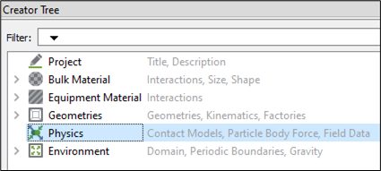
In the Creator Tree, select Physics.
Select Particle to Particle and/or Particle to Geometry from the Interaction dropdown list.
Click Edit Contact Chain at the lower section of the Physics panel.
Under Additional Models, select the FibersBonding checkbox.
Click OK.
The model is displayed in the Model panel.
Select the model and click the icon in the lower-right section of the Physics panel to configure it.

In the Fibers Bonding Model Parameter Editor dialog box, specify values for the following:


For	Specify
Elastic parameters	The following values are used while the bond is within the elastic range: Inner radius - Outer radius ratio: Units: None. Range: [0.0 to 1.0). This value allows you to define the shape of a hollow cross-section of the fiber. If you select 0.0, there is no hollow section. The greater this parameter (0.2, 0.6, 0.9) . the thinner the wall of the fiber. A value of 1.0 would mean that the thickness of the fiber is 0.0. Damping coefficient: Units: s. Range: [0.0, ∞). The greater this value, the stronger the damping. The value corresponds to α_damp. Note: Increasing this value over a certain threshold may require a dramatic decrease of the Time Step if the Damping stabilization parameter is very low. Damping stabilization parameter: Units: None. Range: [0.0, ∞). The greater this value, the more stable the simulation with respect to damping forces. Recommended value: 1.0. If this parameter is set to 0.0, no stabilization is applied and the critical time step may be a lot smaller when Damping coefficient is greater than 0.0. Note: The stabilization method used by this model cannot stabilize a time step bigger than that used with no damping applied, but it can be increased or decreased from the value of 1.0 depending on the need of more stabilization. An excess of stabilization can lead to less damped solutions. Force Stiffness Scaling Factor: Units: None. Range: [0.0, ∞). This value will multiply matrices K₁ and K₂. The value corresponds to α_disp Torque Stiffness Scaling Factor: Units: None. Range: [0.0, ∞). This value will multiply matrices Q₁ and Q₂. The value corresponds to α_rot .
Bond failure parameters	Failure start criterion The elastic range can be limited with several criteria. Once one of these criteria is met, the bond switches to one of the following nonlinear modes: Select None to keep the bond elastic always. If this option is selected, the options in the group Bending behavior beyond failure are ignored. Select Bending-caused stress to establish a stress-based criterion. This criterion uses the value in Maximum stress. Select Bending angle to establish an angle-based criterion. This criterion uses the value in Maximum bending angle. Select Axial stress from force and torque to include axial stresses coming from bending and axial forces. This option ignores shear force and torsion. Select Stress from forces to convert the total force between particles into homogeneous stresses aligned with the force. This option ignores bending and torsional torques, but can mimic a local re-orientation of the bond ('z' shape) wihout the need of very small particles. Select Von Mises stress to approximate Von Mises' criterion to compute a stress value from all sources: axial force, shear force, bending torque and torsional torque. Maximum stress: Units: Pa. Range: [0.0, ∞) In case you have selected Bending-caused stress, this is the maximum allowed axial stress in the section of the fiber, considering exclusively the stresses derived from the bending torque. One this stress value is reached, the bond will act according to the 'Beyond failure point behavior' selected. This value is ignored if you have selected other criteria. Maximum bending angle: Units: deg. Range: [0.0, 180.0) In case you have selected Bending angle, this is the maximum allowed angle for bending between two particles. Beyond this value, the bond will act according to the 'Beyond failure point behavior' selected. This value is ignored if you have selected other criteria. Ignore compression: activate this option if the material you are modeling does not fail under compressive stresses.- Strength variation: Units: None. Use this value to introduce some variation in the strength of the bond (Maximum stress). The value represents the standard deviation relative to the mean value (Maximum stress). Use 0.0 to keep the exact value provided. Post-failure behavior The following options are available: Select Total breakage to completely deactivate the bond once the failure point is reached. Select Constant torque (perfect plasticity) to cap the value of the torque at the level reached when the failure point was hit. The excess of bending (beyond the failure point) will become permanent. Select Constant force (perfect plasticity) to cap the value of the force at the level reached when the failure point was hit. The excess of displacement (beyond the failure point) will become permanent. Select Combined force and torque perfect plasticity to cap the value of a combination of stresses reached when the failure point was hit. The excess of stresses (beyond the failure point) will be converted into permanent relative displacement or relative rotation between the bonded particles. Buckling parameters These set of parameters are used to tune the buckling behavior. Select the folloiwng options: Buckling type Select Buckling (reversible) to ensure that the bond fully recovers its stiffness when unloaded even when it suffers buckling. Select Buckling with damage to ensure that damage is translated into a loss of stiffness with respect to the original one. Since more the bond buckles, the more the damage.The bond will always try to recover the initial relative position of the particles, but with less stiffnes when it is damaged. Select Buckling with plasticity to ensure that buckling is not fully recovered when unloaded. The unloading stiffness of the bond is always constant, but there may be permanent angles which are not recovered and the fiber remains bent. Sample length: Units: m. Range: (0.0, ∞). In a 3-point bending experiment, this is the distance between the supports. Maximum force: Units: N. Range: (0.0, ∞). In the experiment, this is maximum force detected when trying to induce buckling. Minimum force: Units: N. Range: [0.0, Maximum force]. In the experiment, this is the minimum force detected before the slope changes significantly (upwards or downwards). Displacement at minimum force: Units: N. Range: (0.0, ∞). Displacement of the loading edge when the value Minimum force was reached during the experiment. Slope after minimum force: Units: N/m. Range: (-∞, ∞). Slope of the graph after the point defined by the coordinates (Displacement at minimum force, Minimum force).