Joints

Use the Joints tool to create and edit joints.

Joints create lower pair constraints. A constraint is defined as the removal of a degree of freedom (DOF) from a body. Each body has a total of six DOFs, three translational and three rotational.

A lower pair constraint is an idealized form of constraint in which the constraint can be represented by two reference frames (coordinate systems), belonging to two different bodies.

With combinations of constraints in different directions, various types of joints are possible.


Joint Type	Description	Removes Translational DOF	Removes Rotational DOF	Removes Total Number of DOF	Add Friction
Ball	A ball joint (also known as a spherical joint; socket joint) is a three degree-of-freedom kinematic pair used in mechanisms. Ball joints provide three-axes rotation function used in many places, such as steering racks to knuckles via tie-rods and knuckle-to-control arm joints.	3	0	3	Yes
Constant Velocity	A constant velocity joint is a two degree-of-freedom constraint. It constrains the rotation of a body (Body 1) about a specified axis to be equal to the rotation of the other body (Body 2) connected by the joint. The axis of rotation is the Z axes of the markers defined on the connecting user-defined bodies. Constant velocity joints are widely used in drive shafts of vehicles with independent suspension.	3	1	4	No
Cylindrical	A cylindrical joint is a two degree-of-freedom kinematic pair used in mechanisms. Cylindrical joints provide one translation and one rotation function. They are commonly used in many places, such as shock absorber tubes and rods and hydraulic cylinder/rod pairs.	2	2	4	Yes
Fixed	A fixed joint is a zero degree-of-freedom constraint. It applies a rigid connection between the connecting bodies, meaning bodies connected by a fixed joint are forced to move together. Fixed joints can be used to simulate connections where relative displacements are idealized to zero, such as bolted connections, welded connections, and bodies that are fixed in motion and orientation with respect to another body.	3	3	6	No
Planar	A planar joint is a three degree-of-freedom constraint. It constrains a plane on one body (Body 1) to remain in a plane defined on the other body (Body 2) connected by the joint. The planes are defined by the X and Y axes of the markers defining the joint. Body 1 can rotate about Z axis and translate along the X and Y axes of the marker which is used to define the constraint.	1	2	3	No
Revolute	A revolute joint (also known as a pin joint or a hinge joint) is a one degree-of-freedom kinematic pair used in mechanisms. Revolute joints provide single-axis rotation function in places such as door hinges and folding mechanisms.	3	2	5	Yes
Translational	A translational joint is a one degree-of-freedom kinematic pair used in mechanisms. Translational joints provide single-axis translation function in places such as splined shafts and slider mechanisms.	2	3	5	Yes
Universal	A universal joint is a two degree-of-freedom kinematic pair used in mechanisms. It is functionally identical to, and also referred to as a Hooke joint. The only difference between these two joints is the way that the joint is defined. Universal joints provide two rotational functions in applications such as propeller shafts, drive shafts, and steering columns.	3	1	4	Yes
AtPoint	An AtPoint joint is a three degree-of-freedom kinematic pair used in mechanisms. This joint is identical to the ball joint. AtPoint joints provide three-axis rotation function.	3	0	3	No
Inline	An inline joint is a four degree-of-freedom primitive constraint. The constraint is imposed such that the origin of a reference marker on one body (Body 2) translates along the Z axis of a reference marker on the other body (Body 1) connected by the joint. Three rotations are free along with one translation along the Z marker defining the joint orientation. Joint primitives like inline joints may not have a physical existence. They can be used to impose unique constraints where using a regular joint would not be possible.	2	0	2	No
Inplane	An inplane joint is a five degree-of-freedom primitive constraint. It constrains one body (Body 1) to remain in a plane (XY plane) defined on the other body (Body 2) connected by the joint. Three rotations are free along with two translations. The only degree of freedom being arrested is the 'away' motion of Body 1 from Body 2. Joint primitives like inplane joints may not have a physical existence. These joints can be used in applications like imposing geometric constraints.	1	0	1	No
Orientation	An orientation joint is a three degree-of-freedom kinematic pair. The joint constrains the three rotational degrees of freedom while all three translations are free. Effectively, the orientations of the two bodies connected by the joint remain the same.	0	3	3	No
Parallel Axis	A parallel axes joint is a four degree-of-freedom primitive constraint. The constraint is imposed such that the Z axis of a reference marker on one body (Body 2) remains parallel to the Z axis of a reference marker on the other body (Body 1) connected by the joint. All three of the translations are free along with one rotation about the Z axis of the marker defining the joint orientation. Joint primitives like parallel axes joints may not have a physical existence. Parallel axes joints can be used to impose unique constraints where using a regular joint would not be possible.	0	2	2	No
Perpendicular	A perpendicular axes joint is a five degree-of-freedom primitive constraint. The constraint is imposed such that the Z axis of a reference marker on one body (Body 2) remains perpendicular to the Z axis of a reference marker on the other body (Body 1) connected by the joint. All three translations are free along with two rotations about the Z axis of markers on both of the bodies defining the joint orientation. Joint primitives, like perpendicular axes joints, may not have a physical existence. These types of joints can be used to impose unique constraints where using a regular joint would not be possible.	0	1	1	No
Screw	A screw joint is a five degree-of-freedom kinematic pair used in mechanisms. Screw joints imposes a relation between the rotation of one body (Body 1) about an axis to the translation of the other body (Body 2) along an axis. The pitch of the joint completes this relation. One full rotation of Body 1 translates Body 2 by a distance equal to the pitch. Screw joints are commonly used in applications such as bolt and nut constraints and rack and pinion steering.	1	0	1	No

MotionView joints can be set to be compliant or non-compliant. This feature helps in toggling the representation of any connection either as an idealized constraint (Joint) or as a Bushing with stiffness and damping.

Non-compliant Joints: Non-compliant joints act as pure constraints and allow relative motion only between the degrees of freedom of that particular joint type.
Compliant Joints: Compliant joints are identical to bushings and allow relative motion in all six degrees freedom. The relative motion will be dependent on the stiffness and damping of the compliant joint. In order for a joint to be compliant, the Allow compliance option must be enabled at the time of joint creation. A joint created without the Allow compliance option cannot be toggled to be compliant.

Note: The compliance state of joints with Allow compliance within a System can be controlled at the System level.

Create Joints Using the Joints Tool

The following are the standard initial steps to create any type of joint.

From the Model Browser, select the system to which the joint is to be added.
From the Model ribbon, click the Joints icon to invoke the Joints create/edit context.
A Joints guide bar appears (the Body 1 collector is active by default).
- Use the Options menu to Allow Compliance. Otherwise, a non-compliant joint will be created without the ability to change it to compliant.
Optional: Select the Create Pair check box below the guide bar to create a Joint pair.
An entity pair is a combination of two entities of the same type within a single definition. It has two sides, “Left” and “Right”. Entities with properties can be marked as Symmetric with one side as the Leading side. The other side then becomes the Following side. The properties of Following side are reflected from the Leading side across the Global X-Z plane.
Resolve the Body 1 collector by clicking on a body graphic in the modeling window or by using the Advanced selector .
The selected body should now be highlighted in red.
Similarly, resolve the Body 2 collector by picking a different body.
The selected body will be highlighted in blue.
Resolve the Origin collector using one of the following methods:
- Click on an existing point in the modeling window.
- Hover and click on a CADGraphic location (an edge corner, center, or surface center). A new Point will be created at this location.
- Use the Alt key to highlight the mesh of a CADGraphic or FileGraphic. Hover and click on a node. A new Point will be created at this location.
- Use the Advanced Selector to pick an existing point.
Click the Play button or the Create button on the microdialog to create a joint with the selected body and point references.

Note: Once the joint is created, it is in Edit mode with a microdialog displayed near the joint.

Edit Joints

Joint references and orientation can be edited in two ways.

Using the guide bar and microdialog:
1. Select the joint to be edited and click on the Joints icon in the Model ribbon. The joint is in edit mode with the guide bar and microdialog visible.
2. To change the Body references and Origin, activate the collector in the guide bar and pick from the modeling window or use the Advanced Selector.
3. Joint Type can be changed in the microdialog. Select the required joint type under the Joint Type option.
4. Use the Swap bodies icon to swap around the Body 1 and Body 2 references among the selected bodies.
Note: The Orient Axis icon appears on the microdialog if it is applicable to the selected joint type in the case of non-compliant joints or any joint that is set to compliant.

To orient the joint, click the Orient Axis button to enter the Orientation context.
Using the Entity Editor:
1. Select the joint to be edited. Its properties will appear in the Entity Editor
2. To change the Body references and Origin, activate the collector in the Entity Editor and pick from the modeling window or use the Advanced Selector.
3. Orientation can be changed using the Orientation section.

Joint Properties


Property	Description
General
Label	Descriptive label for the entity.
Varname	Variable name of the entity.
ID	Integer identifier.
Active	Active state of the entity. True or False. Entity is deactivated if False.
Body 1	First body of the joint.
Body 2	Second body of the joint.
Origin	Origin of the joint.
Type	Type of joint.
Compliant	Compliance state of joint. True or False. Joint is compliant if True and represents a bushing. This property is visible when the joint is created with Allow Compliance option.
Orientation	Use this section to orient the non-compliant joint. Types and methods of orientation depend on Joint Type.
Alignment Type (Type 1 \| Type 2)	Applicable for Universal, Inline, Inplane, Planar, and ParallelAxes only. Select the type of alignment desired. Refer to the comment below.
Method (Method 1 \| Method 2 )	Method of orienting the axis or axes of the joint. Available choices are Point and Vector.
Point\|Vector	Select a Point or a Vector based on the Method selected. The joint will be oriented along the direction of the point or the vector from the Origin.
Note and Tags
Note	Optional descriptive note.
Attachment Candidates	Add tags for the entity to use as possible attachments to Systems/Assemblies/Analyses.

Note: Properties of compliant joints are the same as Bushing properties.

Note on Non-compliant Joint Orientation

By defining a joint between two bodies (referred as I Body and J Body), the constraint between the bodies is imposed using two markers or coordinate systems (I Marker and J Marker) belonging to each body. By orientating a joint, these markers are oriented in certain directions along or about which the joint has degrees of freedom (usually Z axis of the markers).

Figure 1. Z Axes of the revolute joint oriented along a point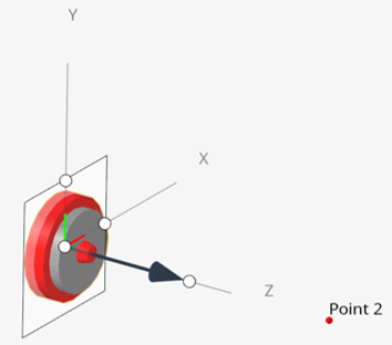

Revolute | Translation | Cylindrical – The orientation causes the Z axes of these joints (direction of DOF) to be aligned in the given direction.

Alignment types

Certain joints have different ways of alignment based on the joint type.

Universal joints can be aligned either by aligning the Shaft direction or the direction of the Crosspin (which is perpendicular to the shaft and part of the yoke) on either side.
Inline joints can be aligned by either aligning the axis along a point or a vector or providing another origin Origin 2.
Inplane, Planar, and Parallel axis joints can be aligned by either specifying the normal to the plane (a point or a vector) or defining the plane with two inputs using points or vector.

Adding Friction

Friction can be added to the following non-compliant joints - Ball, Revolute, Translation, Cylindrical, and Universal.

MotionSolve uses the LuGre (Lundt-Grenoble) model for friction. Refer to the MotionSolve Force_JointFriction modeling statement for additional details.

To turn on friction:

Activate the Use Friction check box under the Friction section in the joint’s Entity Editor. The Friction Properties are now listed.
Specify the friction coefficients, Effect options, geometrical parameters, and LuGre parameters.

Note: Coefficients and parameters that are applicable vary based on the type of joints.

Friction Properties


Property	Description
Friction
Use friction	Add friction to the joint.
Dynamic friction coefficient	Coefficient of friction in the dynamic regime.
Static friction coefficient	Coefficient of friction in the static regime.
Stiction transition velocity	Velocity at which the friction regime transitions from stiction to dynamic friction.
Use for static analysis	Turn on/off friction during static analysis.
Effect	Effects to be included - Stiction, Sliding or both Stiction and Sliding.
Input Forces	Control which forces among Preload, Reaction forces, Bending moment (where applicable) are considered to calculate friction.
Pin radius	Radius of pin for friction on revolute, cylindrical, and universal joints.
Ball radius	Radius of ball for friction on ball joint.
Torque preload	Preload friction torque for revolute, cylindrical, universal, and spherical joints.
Friction arm	The moment arm used to compute axial friction torque in revolute and universal joints
Bending arm	The moment arm to compute the bending moment in revolute and universal joints.
Force preload	The preload friction force for translational and cylindrical joints.
Initial overlap	The initial overlap of the sliding parts in translation and cylindrical joints.
Reaction arm	The moment arm of the reaction torque about the translation joint axial axes.
Overlap delta	Describes whether overlap in the sliding joints (Cylindrical and Translation) increases or decreases on movement of the joint along the positive direction of the Z axis.
Rotation constraint	Applicable for Universal joint. Select I Yoke or J Yoke to add friction to the first or second DOF axis respectively. Select Both to add friction on both axes.
LuGre parameters
Bristle stiffness	Specify the bristle stiffness in the LuGre model. This models the stiffness resisting micro-deformation in the friction element.
Damping Coefficient	Specify the damping coefficient for the pre-displacement (or stiction) regime to damp out the bristle vibrations in the pre-displacement regime.
Viscous Coefficient	Specify the coefficient for the viscous damping force that occurs when relative sliding begins. This is responsible for the increase in friction force with the increase in the slip velocity.