Frequency Response
![]()
Frequency Response Analysis
Frequency response analysis is a method to find the response of a structure subjected to frequency dependent loading. Frequency response can be determined by two methods namely Direct Frequency response and Modal Frequency response analysis. The direct method calculates the response directly in terms of the physical degrees of freedom of the model. The modal method calculates the response based on the Eigen values and Eigen vectors obtained from normal mode analysis. The modal method is computationally cheaper than the direct method.
Features available in SimLab Frequency Response Analysis
- Multi Nodal Input Excitation can be applied.
- Multi Nodal Response can be obtained
- Frequency dependent pressure excitation can be applied.
- Frequency vs. Transfer Function plots can be visualized.
- Frequency vs. Response plots can be visualized.
- Export of Calculated data in csv format can be done.
Methodology adopted in SimLab
Modal Frequency response method is followed in SimLab. SimLab needs a Normal Mode analysis result file to proceed with the Frequency Response Analysis. SimLab supports only for Nastran, Abaqus and Permas Normal mode analysis results file. There are two ways to perform the Frequency Response analysis in SimLab. They are
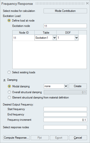
- Define load at node Method
The Excitation loads can be applied on the nodes directly in the Results workbench by selecting the nodes and defining the frequency dependent excitation table for each node.
- Select existing loads Method
The Excitation loads can be defined in the Structural workbench and those defined loads can be referred in the Frequency Response dialog and the frequency dependent excitation table can be defined for each load. Only Force and Pressure loads defined in the Structural workbench can be referred for Frequency Response calculation.
Definition of terms in Frequency Response Dialog
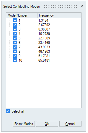
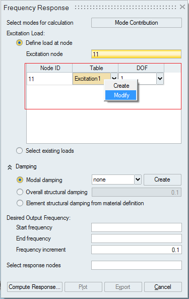
- Select modes for calculation:
The contribution of modes in frequency response analysis can be controlled by this option. User can decide which modes can be taken into account for the analysis. Also the user can change/adjust the frequency value using this option. During analysis, the modes will have the edited frequency value and all other parameters such as modal mass, stiffness remains the same as read from results file.
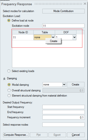
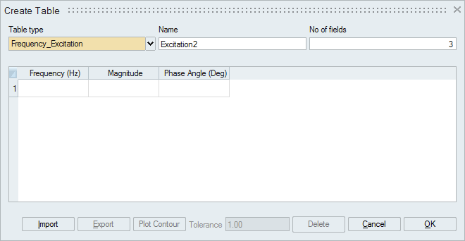
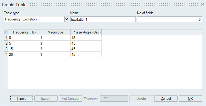
- Excitation Table:
It is used for defining the loading function. The load must be defined as a function of frequency. Excitation table can be defined using the following options,
- Excitation table can be created using Right click in the table cell → Create
option
-
Excitation table can be modified using Right click in the table cell -> Modify option
- Excitation table can be created using Right click in the table cell → Create
option
- Damping Table : It is used for defining the Modal damping. The damping ratio is defined as a function of frequency in this table.
- Frequency Range : It is used for defining the Frequency range within which the Excitation should happen. The lower limit of the frequency range should be specified in the Start Frequency and upper limit of the frequency range should be specified in the End Frequency.
- Frequency increment : The intermediate frequencies of interest within the frequency range are obtained by this parameter. The frequency values gets incremented by this value from the lower limit till the upper limit.
Inputs : (For Define load at node Method )
- Range of Forcing Frequencies - The lower and upper limit of the frequency range.
- Frequency Increment.
- Excitation nodes for Define load at node Method
- For Each excitation node - a Excitation table and Degree-of-Freedom has to be defined .
- Damping - Either Modal Damping (Damping values are Frequency dependent) or Overall Structural Damping Factor (OptiStruct Equivalent – PARAM,G ) can be specified.
- Response nodes.
- Element structural damping from material definition is supported only for OP2 file. This value is read from OP2 file. For other result files, output will be as same as undamped vibration.
- If the selected excitation node is from RBE body, The element structural damping is zero. If damping needs to be accounted for computation, use structural damping coefficient.
Output
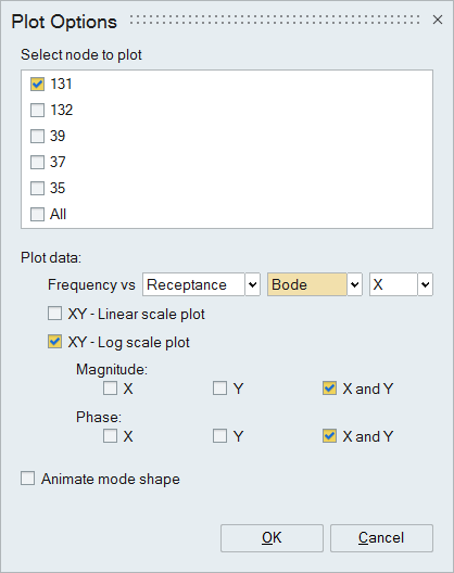
- Transfer Function(Frequency Response Function) plots
- Frequency vs. Receptance
- Frequency vs. Mobility
- Frequency vs. Accelerance2.
- Frequency Response plots
- Frequency vs. Displacement
- Frequency vs. Velocity
- Frequency vs. Acceleration
- Stress Response plots
- Frequency vs. Normal Stress
- Frequency vs. Shear Stress
The plots are available in Linear as well as Logarithmic scale. The various scale options available are:
- Both Linear
- Both Logarithmic
- X Logarithmic
- Y Logarithmic
Bode Plot is supported.
Multiple Response Curves in a single plot is also supported.
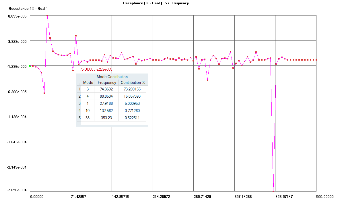
Picking in Frequency response plot displays first five contribution modes along with the contribution percentage in tabular form.
Animation supported for the contributing modes. For this, Animate mode shape toggle should be turned on in Plot Options dialog. If mode number in the Mode contribution table is selected, animation of the corresponding mode shape can be visualized. The mode also updated in graphics and in Results browser.
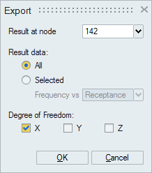
Export
The calculated data can be exported in csv file format. Various export options are available and the user can select the required format and then export the data.
 Steps : (For Define load at node method)
- Import the Normal Mode analysis Nastran/Abaqus/Permas results file.
- In the Frequency response dialog, enter the Range of Forcing frequencies and Frequency increment.
- Select the Input Excitation nodes. For each Excitation node , define the excitation table ( Frequency-Magnitude-Phase ) and the degree-of-freedom.
- Specify Modal damping ( Frequency vs. Damping Ratio ) or Overall structural damping factor or Element structural damping from material definition if needed.
- Select the response nodes by setting the focus on output nodes option.
- Then click on Calculate.
- Click Plot button to view the various transfer function and frequency response plots.
- Import the Normal Mode analysis Nastran/Abaqus/Permas results file.
- Define the necessary Force and Pressure loads in the Structural Workbench.
- In the Frequency response dialog, enter the Range of Forcing frequencies and Frequency increment.
- Select the loads defined in the Analysis workbench by picking the loads in user interface.
- For each load , define the excitation table ( Frequency-Magnitude-Phase ).
- Specify Modal Damping ( Frequency vs. Damping Ratio ) or Overall Structural damping or Element Structural Damping if needed.
- Select the response nodes by setting the focus on the output nodes option.
- Then click on Calculate.
- Click Plot button to view the various transfer function and frequency response plots
Sample Frequency response Plot