Plot
![]()
Plot
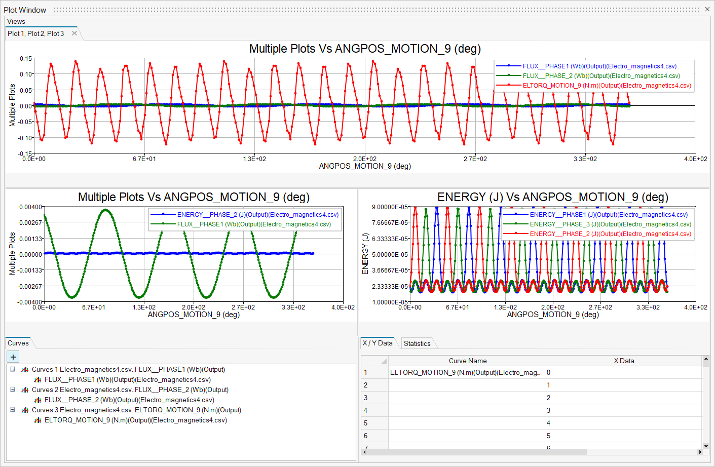
This tool is used to display graphs for selected results components.
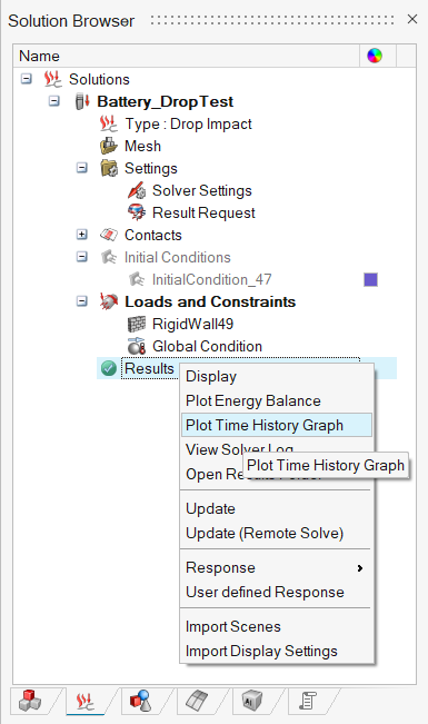
Solution Method: Users can view the "Plot Time History Graph" option in the results right-click option from the solution browser.
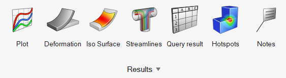
Direct Method:Users can view the plot tool in the Results menu as a ribbon. Users can load result files directly by this method .
Enhanced Plot GUI to list the Data types and Result components on the X and Y axes, in the library structure.
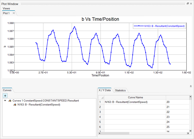
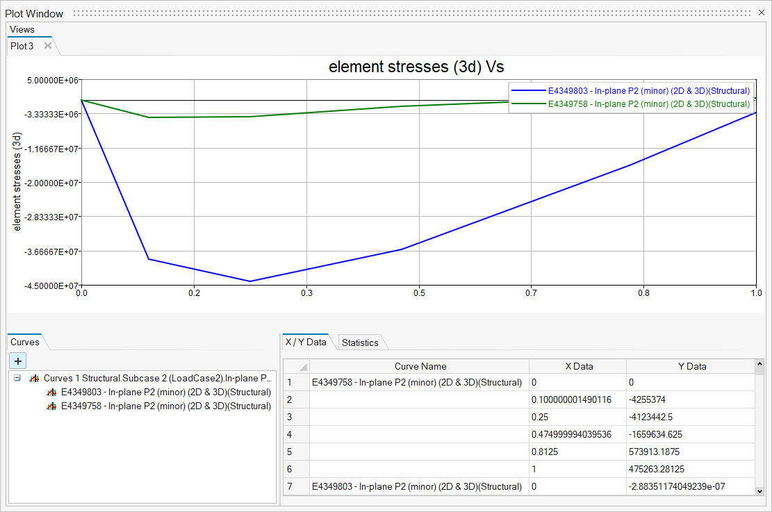
New empty plot window will be created when Plot tool is clicked.
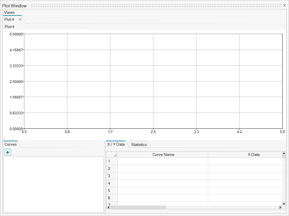
Curves Tab is supported.
+ symbol is used to open the Create Curve dialog and add curves to the plot.
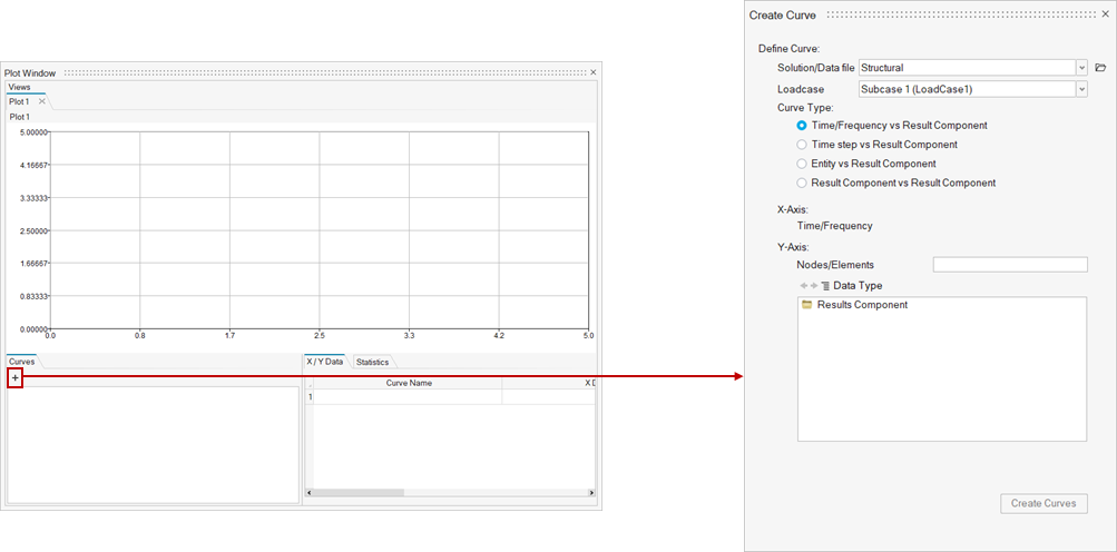
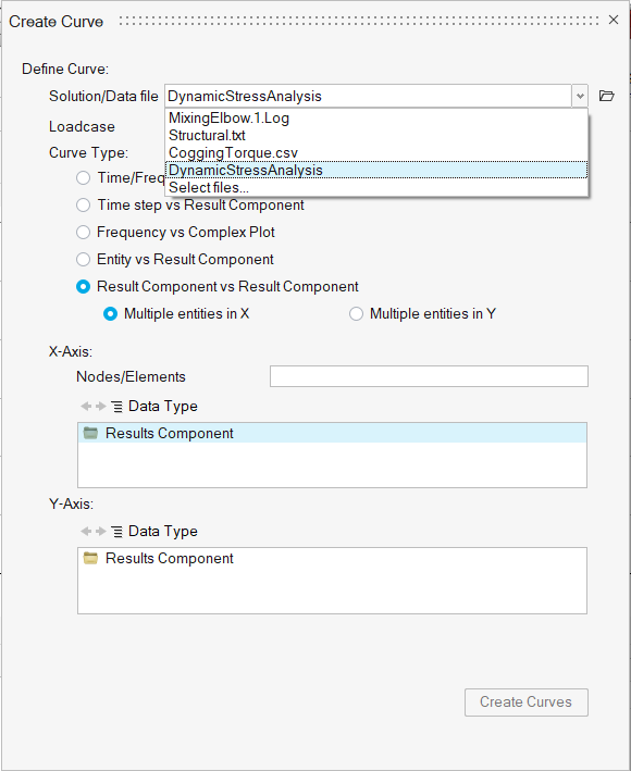
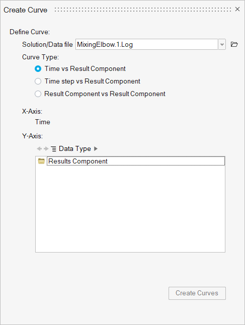
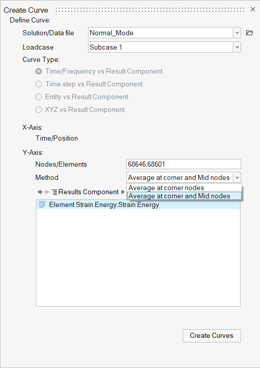
Create Curves:
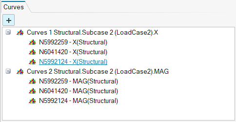
This option is used to create and display the new curves and add them to the plot. The curve objects can be visible in the curves tab.
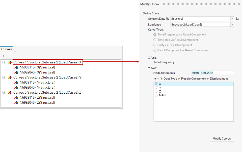
Double click on a curve is used to open the “Modify Curve” dialog. This mechanism can be used to modify a curve or to review its definition.
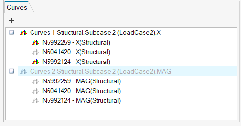
Toggle on/off is used to show/hide the curves.
The following file formats are supported. Log, csv, txt and xml.
Solution/Data File Option
-
All the available results are listed in the Solution/Data file dropdown. The selected result file will be loaded and made available for plotting.
- Users can also bring in the results from external files from the "Select files” option. The following formats .log (AcuSolve) files, csv (FLUX) files and txt(nFx) files are supported.
- This option also allows the import of the XML file to draw the graph in the
plot window.
File Import / Select File:
This option allows the user to import the files directly and view the graph for imported components. Users can import log files, txt files and import multiple CSV files directly in this method.
Users can “Select files…” option in the Solution/Data file list to import the results file directly.
-
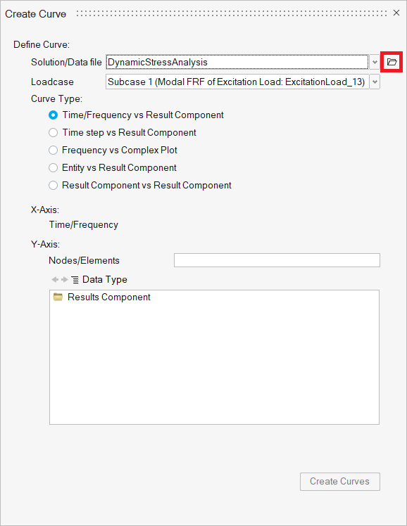
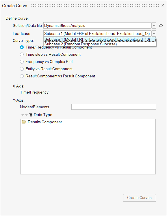
The Load Case option is visible for the H3d results file that has more than one load case.
- Support to select load cases for all the solutions
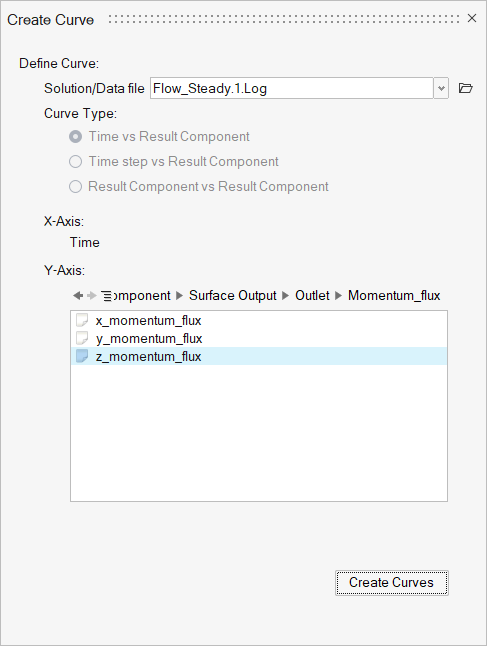
- For log(Acuolve) files
- Time/Frequency vs Results Component
- Time Step vs Results Component
- Results Component vs Results Component
- For Flux Solutions
files
- Time/Position vs Global Quantities.
- Time/Position vs Results Component
- Entity vs Results Component
- Results Component vs Results Component
The Curve types will be displayed based on CSV and H3D files in the results folder.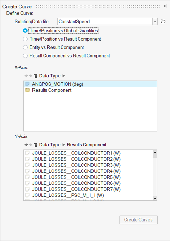
- The "Time/Position vs Global Quantities" option will be displayed for the CSV file located in the results options. This curve option will load the CSV file when selected.
- H3D files will be loaded for other curve-type
options.
Input:
Output:
- For H3d files
- Time/Frequency vs Results Component
- Time Step vs Results Component
- Frequency vs Complex Plot
- Entity vs Results Component
- Results Component vs Results Component
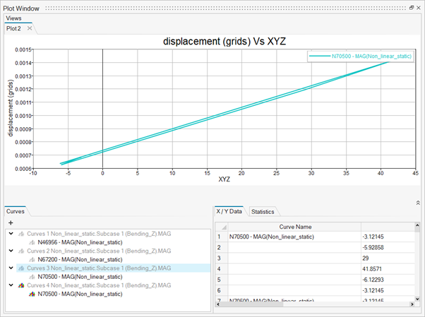
- XYZ vs Results Component
-
The plot tool contains the following selection options for CSV files.
- Input:
- Output:
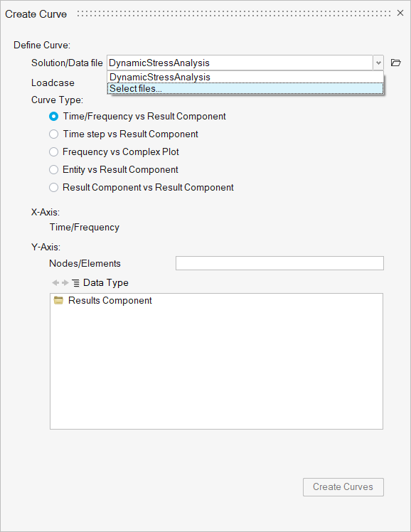
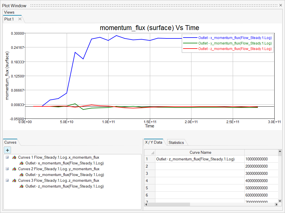
Time/Frequency vs Results component
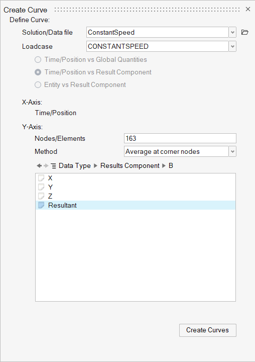
- Time/Frequency vs Result component is used to plot the time history for AcuSolve and H3d results files.
- X axis is time and Y axis component is selected based on entity selection. Results components are listed based on the selected entity (node/element).
- The Selected entities are listed in the Nodes/Elements on the Plot dialog.
- Input:
- Output:
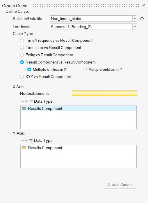
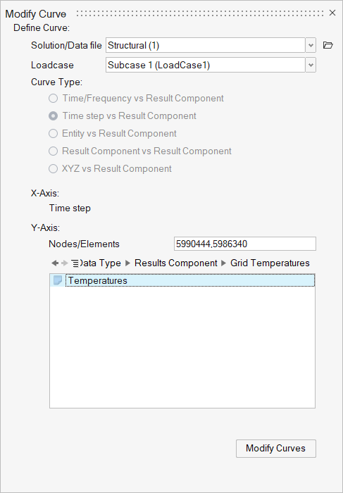
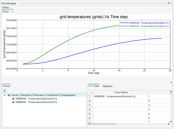
Time Step vs Results component
- Time Step vs Result component is used to plot the time step vs results for nonlinear static analysis.
- X axis is time and Y axis component is selected as same as the time history plot.
- Input:
- Output:
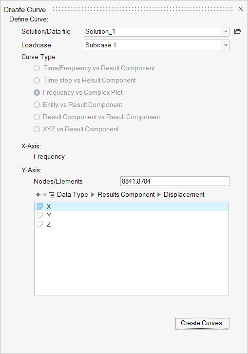
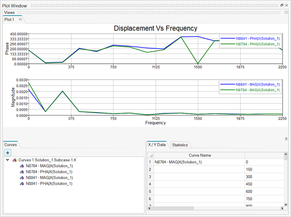
- Frequency vs Complex Plot option is used to plot Magnitude (or Real) and Phase (or Imaginary) data for H3d results files.
- X axis is always frequency and Y axis component is selected based on entity selection. Results components are listed based on the selected entity (node/element).
- The Selected entities are listed in the Nodes/Elements on the Plot Dialog.
- Note: If the model contains Phase and Magnitude components then it will display the “Frequency vs Complex Plot”
option otherwise this option will not show in the dialog.
Input:
Output:
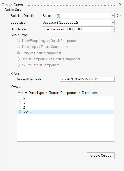
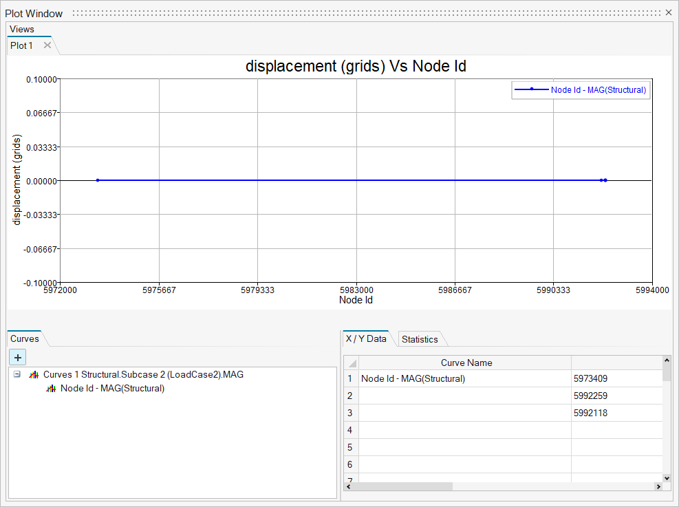
Entity ID vs Results component
- Entities can be selected directly by picking entities on the graphical screen.
- The X axis is entity IDs, and the Y axis component is selected based on entity selection.
- Node path options will be visible in the X-Axis only if that model has Node Path bodies.
- Input
- Output:
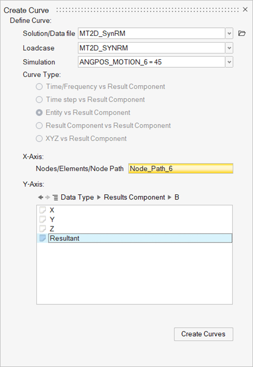
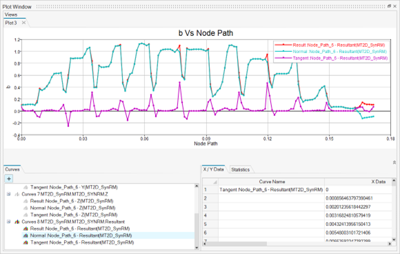
Node Path:
- The Node Path option will only be displayed if the modal has node path bodies. Otherwise, the label of the node path won't be shown in the X-Axis label.
- The Results component will be displayed in the Y-Axis only if that component has sub-components like X, Y, Z, and Resultant.
- The User will create three curves for magnitude, Normal, and Tangent for the selected node path body.
- In the X-Axis, the User will display values of the absolute distance between the first node to other nodes present in the selected node path body.
- Input:
- Output:
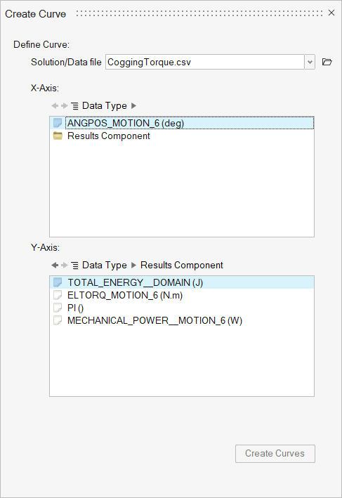
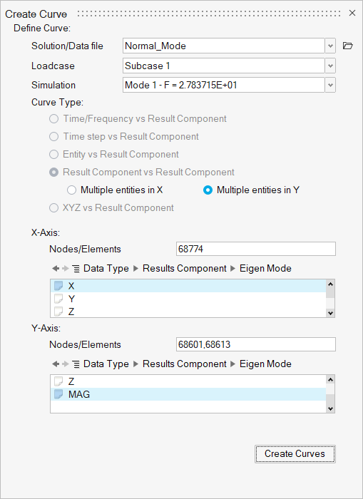
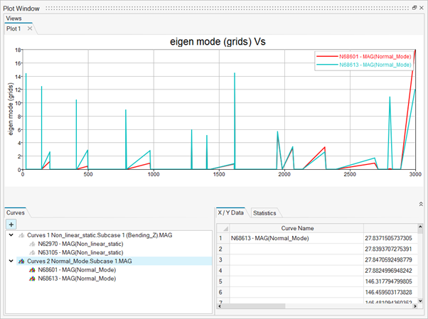
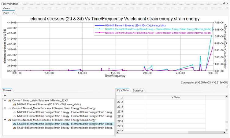
Results component vs Results component
- Entities can be selected directly by picking entities on the graphical screen.
- Both X-axis and Y-axis components are selected based on entity selection.
- This curve type is removed for “Average at corner nodes” and “Average at mid and corner nodes” options.
- Input:
- Output:
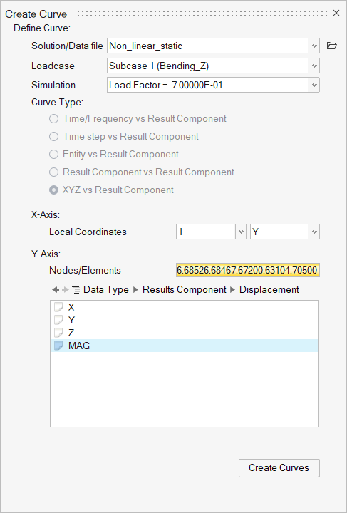
XYZ vs Results component
- Enabling this option displays the local coordinate option on the X-axis and lists all defined local coordinates for plotting.
- Input:
- Output:
“Average at corner nodes” and “Average at corner and mid nodes” options
- These two options will be displayed only if the model has nodal
results.
Input:
Output:
- These two options will be displayed only if the model has nodal
results.
Solution Browser:
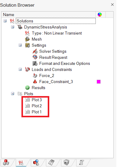
- A single click on the plot/curve icons in the browser is used to show/hide plots.
- The plots and curves data are saved with slb as xml files so that the user can open the slb, and automatically plots get loaded along with slb. The plots and curves are maintained for each database.
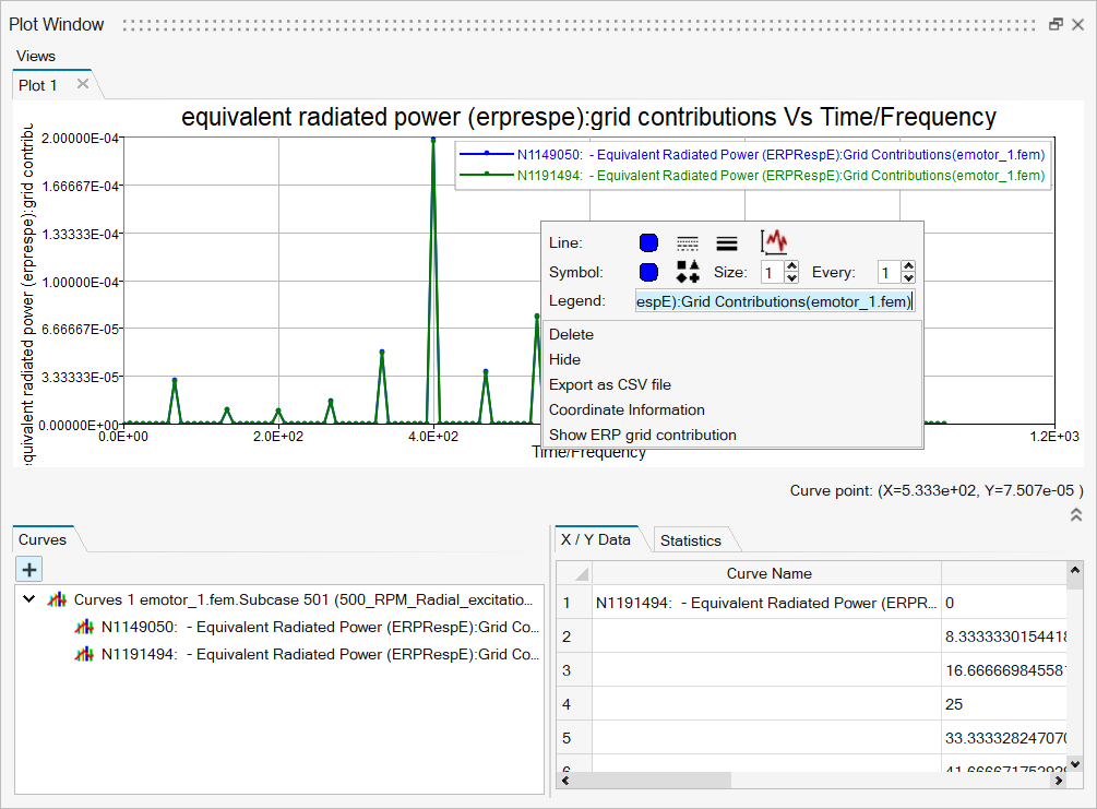
Shift + RMB (Right Mouse Button) options on the curve:
- Delete
- Hide
- Export as CSV file.
- Coordinate Information
- Show ERP grid contribution
Delete Curve:
- This option uses to delete selected curve on the plot Window.
Hide Curve:
- This option uses to hide selected curve on the plot Window.
Export as CSV file:
- This option uses to export the curve data in the CSV file format.
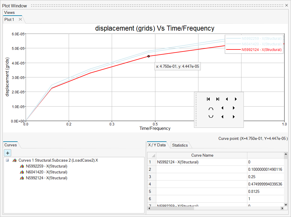
Coordinate Information:
- Choose the Coordinate Information option to view the coordinate micro dialog.
- Press escape key to close the coordinate information micro dialog.
Show ERP grid contribution:
- Displays the ERP grid contribution contour plot at the selected frequency.
- This works only when ERP grid contribution curve is available in the.h3d file.
Peak points:
Peak points have various options that users can switch next coordinate points, previous coordinate points, switching between maximum peak points and least peak points. Also, it shows the coordinated values of all the plotted curves.
Shift + RMB (Right Mouse Button) options on the empty space of plot window.
- Export 2D plot
- Hide all Curves.
- Display all Curves.
- Delete all Curves.
- Show table.
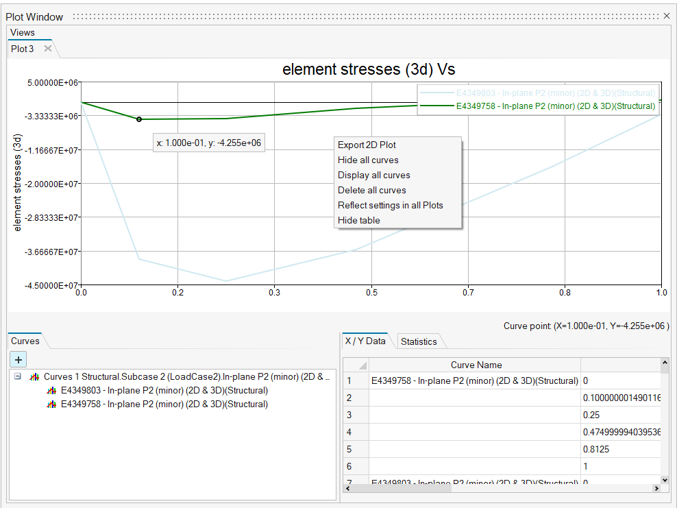
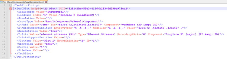
Export 2D Plot:
- This option uses to export 2D Plot in XML format. It exports data only for the
current plot window.
Hide all curve:
- This option is used to hide all the curves on the active plot window.
Display all curve:
- This option is used to show all the curves on the active plot window.
Delete all curve:
- This option is used to delete all the curves on the active plot window.
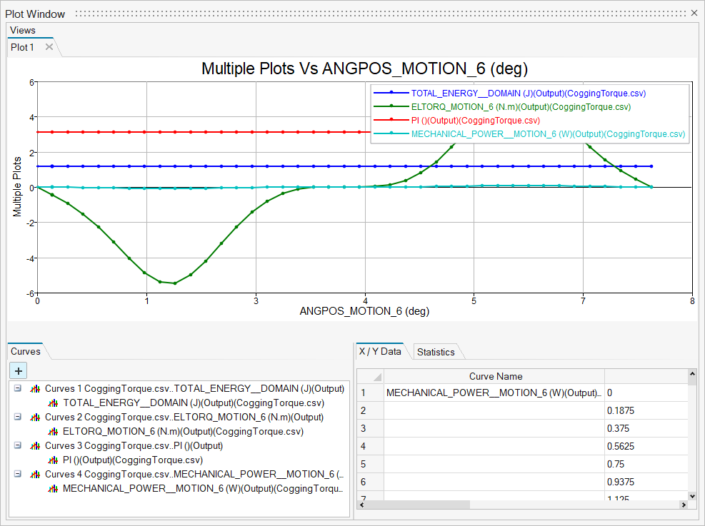
Show/Hide table option:
This option is used to show and hide the X/Y data table and Statistics table.- X / Y Data table:
- View the values of X and Y coordinates of all the curves of the current plot window.
- Statistics table:
- View the values of statistics output like RMS, Min, Max, Median, Delta, Centroid, Mean, Variance, Skewness, Std.Dev, Avg.dev and Zero Crossings.
Tile View:
- Users can view the multiple plot window in the same window.
- Tile view icon appears when moving mouse cursor right most top.