How to create a Magneto-Mechanical Topology Optimization solution?

Introduction

Despite its diverse underlying principles, topology optimization may be regarded as complementary technique and belong to the same framework of structural optimization method offered in SimLab. Common tools for the description of an optimization problem is shown in the following photo. These are accessible through the Analysis menu.

Topology optimization strategies implemented in SimLab

Two well-known topology optimization strategies for electromagnetic devices are available in SimLab through the OptiStruct Solver, namely:

the Density method and
the LevelSet method (it is advised for electric motors).

For an introduction on these gradient-based methods, please refer to the following open access references: https://ieeexplore.ieee.org/document/9888100

Steps to create a Topology Optimization Solution

The workflow definition of a Magneto-Mechanical Topology Optimization Solution is as follows:

Step 1 - Geometry & Meshing

Magneto-Mechanical Topology Optimization is based on Finite Element Analysis. Therefore, the first step to perform Optimization is to define the geometry of your electrical machine and a mesh. Please follow the following instructions & hints:

Create your 2D geometry in SimLab as CAD bodies. You can either define it using SimLab modeler or import it. If you start from an existing device, you may need to adapt the geometry of regions you plan on optimizing (remove holes, simplify corners).
Create mesh bodies based on these CAD bodies. You can use the Motor Mesh tool to easily build a proper mesh for Electromagnetic finite element analysis, including mesh symmetries.
Adapt the mesh of the regions of optimization. It is advised to use a fine and regular mesh in those regions. In SimLab, this can be achieved easily using a “Surface Mesh” control.

Step 2 – Define an Electromagnetic Solution

To optimize the magnetic torque of your device, it is required to define an electromagnetic study on the previously meshed bodies. This study must be a 2D Magneto Static or Transient Magnetic analysis. Please refer to Current limitations to get a detailed view of current limitations imposed on the Electromagnetic Solution for optimization.

Note: Parametric Distribution applies in Magneto Static applications. It is advised to use the Parametric Distribution feature to speed up computations. You can refer to Format and Execute Options for more information.

Before going to Step 3, it is advised to:

Take the time to solve your Electromagnetic Solution and check its results & physical validity.
As you may want to later launch optimizations with different targets and settings, it is advised to save this validated study in a dedicated “EM study” SimLab database, and to use the “Save As” action to start the next Step in another database.

Step 3 – Define a Structural Solution

To get the best result out of topology optimization of electrical machines, it is needed to add mechanical targets in the optimization. This requires defining mechanical study in SimLab. It is advised to define this study on the same meshed bodies as the Electromagnetic Solution. Mechanical studies can be defined using Structural Solutions. In SimLab, there is a wide range of available mechanical models. For EM/Structural optimization, only the following types of analysis are allowed:

Static Stress (Linear or Non-Linear Static) Solution
Dynamic Stress (Normal Mode) Solution

In terms of mechanical loads & boundary conditions, SimLab offers a lot of possibilities that can be used as needed, if you stick with those three previous kinds of analysis. This definition is case dependent, and you will find learning resources here.

To help you discover the EM/Structural optimization feature, here is a description of a typical Linear Static analysis under centrifugal load. This is a good starting point to try to optimize a rotor.

Create the Structural Solution on the rotor part
Assign mechanical properties to your material and bodies
Create and assign a cylindrical Coordinate system, a Body Force centrifugal Load and some Constraints to model your boundary conditions
Solve the Solution to check results before moving to next step

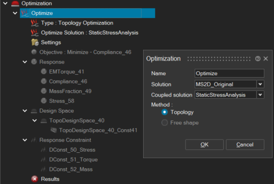
Step 4 – Create an Optimization Solution

It is now time to define your Optimization Solution. In the Optimization Solution creation window, please select the Electromagnetic Solution defined at step 2. Then, please select as “Coupled Solution” the Structural Solution defined at step 3.

Starting from this point, the definition of the EM/Structural optimization follows the general rules of the Optimization Solutions in SimLab (Optimization). Learning resources can be found in (https://web.altair.com/altair-for-simlab-learning-center-trls). As a starting point, here is a general overview of the different elements that need to be defined in the Analysis panel:

Design Space can be used to define the bodies you want to optimize. It must be a region defined as a Soft Magnetic material in your Electromagnetic Solution. For more information: Current limitations. In this dialog box, you can also select the LevelSet option which is strongly recommended for EM/Structural topology optimization.
Design Constraint allows you to add geometric constraints to your Design Space. This includes design thickness constraints, symmetries, manufacturing constraints, etc.
Response is where you define the relevant physical targets of your Optimization. In SimLab, you have access to a wide range of Responses, but the most important ones in our case are the following:
- Electromagnetic Torque Response – computed from the Electromagnetic Solution defined at step 2, this is the most important Response for EM/Structural optimization
- Volume, Mass fraction and Mass – those responses can be defined to control the maximum amount of material allowed in the Design Space at the end of the optimization
- Static Stress of homogeneous material – this response gives the opportunity to optimize the Design Space with respect to the stress on the material
- Compliance – the sum of strain energy in your model.
Objective & Constraints – are needed to define the effective targets of the Optimization for each previously defined Responses
Solver Settings – can be used to refine solvers options. The following modifications are suggested compared to default option values:
- Maximum number of iterations is suggested to be 80.
- Improved discrete topology optimization is suggested to be set “True”.