Magnetostatic Integral solution

Solutions > Electromagnetics > Magneto Static

Introduction

The Magneto Static Integral solution allows the user to study the phenomena created by a magnetostatic field. The magnetic field is related to the presence of DC currents (stationary currents) and/or of permanent magnets.

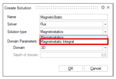
Note: For more information about the Magneto Static Integral workflow, please consult Magnetostatic Integral.

Solution dialog box

The Magnetostatic Integral solution is available only in 3D domain.

In Magnetostatic Integral containing Motion load, once the Motion load is created, the solution dialog box is updated with new inputs: the Motion parameters to pilot the position of the moving bodies during the solving:


Solution piloted by a Monovalue	Solution piloted by Multivalues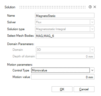

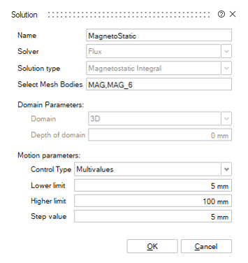
Monovalue allows to solve with the entered position. Multivalues allow to solve with the position varying from a Lower limit to a Higher limit with a Step value. For more information on the Motion, please refer to MSIM Motion.

Application example

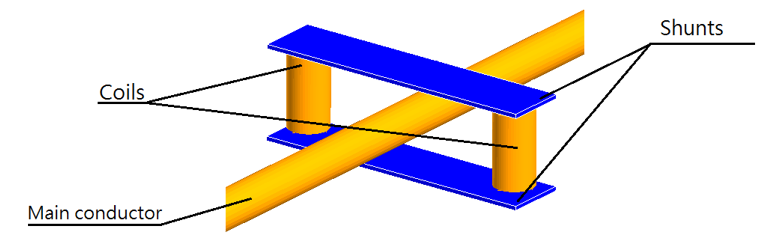
Study of a current sensor

This example shows the advantages of the integral method compared to the conventional finite element approach for a current sensor. In this case, a current is injected into the main conductor and we are looking to compute the magnetic flux observed by the auxiliary coils, as shown in Figure 1. The characterization of this sensor requires knowledge of its gain and crosstalk.

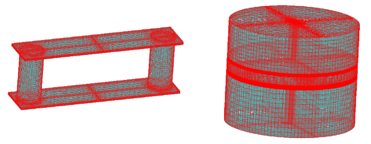
This device being characterized by a large quantity of leakage flux and by the distances between the conductors that can be large, the use of the conventional finite element method requires to intensively mesh the surrounding air. To get results approaching the real the solution, the mesh must be symmetrical and very dense, which increases the computation time (see Figure 2).

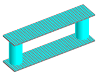
Figure 2. On the left, the mesh of the device. On the right, the mesh of the air.

The integral method is much cheaper in terms of meshing elements because we do not mesh the air anymore (see Figure 3).

Comparison of the two methods:

Table 1. Computation time for one value of current in the main conductor
Method	Mesh	Solving	Magnetic flux computation
Integral	2 s	30 s	1 s
Finite elements	20 min	5 min	20 min

For the computation of the flux in a coil, the volume integral method is also faster than the finite element method. This magnetic flux is split into two contributions, the contribution of the other coils and the contribution of the magnetic parts [2]. In the air and for the other coils we compute the magnetic flux by a Biot & Savart law. For the magnetic parts the computation is done with the magnetic vector potential already computed in resolution.

Results

The study of this sensor requires to know its gain defined in the frequency domain by the following relation:

with

: the frequency
: the current in the main conductor
: the magnetic flux in the auxiliary coils

We can compute the gain for several values of current:

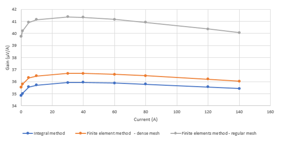
Figure 4 shows that the finer the mesh is, the more the results will be close to the real solution and therefore to the solution provided by the integral method.

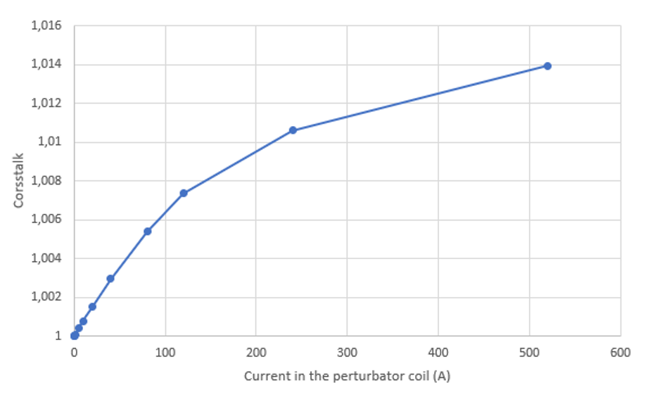
A complete study also requires knowing the crosstalk of the sensor:

with

: the gain corresponding to the sensor with an offset on the position of the main conductor.

Note: Total simulation time with the integral method for this study: 15 minutes.

Note: Total simulation time with finite element method with dense mesh for this study: 6 hours.

References

[2]: L. Huang, G. Meunier et al., "General Integral Formulation of Magnetic Flux Computation and Its Application to Inductive Power Transfer System," IEEE Trans. on Mag., vol. 53, no. 6, pp. 1-4, June 2017.