Solver Settings

Introduction
This tool is used to define Flux PEEC solver settings. The settings affect the physics and the resolution techniques for Parasitics Extraction solution.
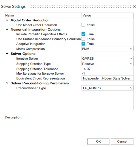
Model order Reduction
- Use Model Order Reduction: By default, this option is unchecked
(False). It allows the solver to generate a reduced
model using the Model Order Reduction method, then perform the computation on
all frequency steps. This option is really interesting because of the
computation time it saves, and a high number of frequency steps can be defined
for better interpolation of results within a frequency range.Note: This method only works when using the "state" solvers in the "Equivalent Circuit Representation" option.Note: The export of the reduced model is not available.Important: The Model Order Reduction option doesn't work when the Surface Impedance Boundary Condition option is enabled.
- Expansion points stopping criterion: By default, it is set to 1e-3. This criterion is defined as a relative error of a Krylov space vector norm between a new expansion point and the previous expansion points already calculated in the order reduction of the model. This relative error shows the impact of the added expansion point on the entire system.
Numerical Integration Options
- Include Parasitic Capacitive Effects: By default,
this option is checked ( True). It allows to take
into account the capacitive effects in the geometry due to potential
differences. These effects are considered in addition to the resistive and
inductive effects which leads to a full RLC model. If the option is
unchecked (False), the model will consider only RL
(resistive and inductive) effects. Note: Remember that delay effects related to wave propagation are neglected.
-
Use Surface Impedance Boundary Condition: By default, this option is unchecked (False).
Surface Impedance Boundary Condition (SIBC) enables the modeling of volume conductive and/or magnetic regions in order to efficiently simulate various devices with only a boundary surface mesh when the skin depth allows it (see below). The computational effort is considerably reduced in comparison with volume approaches.
Note: From experience, the thickness of the device from which the method is very accurate should be seven times greater than the depth of the skin. For example, if you have a copper layer 1 cm thick, the method is more accurate after 2.2 kHz, but of course, this is not a general rule. Favor its use at high frequency.This option applies to all the solid bodies of the solution. An update will be done in the future versions in order to be able to select manually the bodies where the SIBC will be applied.
Important: The Surface Impedance Boundary Condition option doesn't work when the Model Order Reduction option is enabled. - Adaptive Integration: By default,
this option is checked (True). It improves the
calculation of the integrals of parasitic inductances and capacitances. It
uses an adaptive Gauss point algorithm to ensure good integral accuracy on
every interaction between two mesh elements. This option can lead to
additional calculation time.Important:
- For Tetrahedral mesh, this option can be unchecked (False) to save lot of calculation time, and the lost precision is negligible.
- For hexahedral mesh, it is recommended to leave this option checked (True) to obtain correct results; unchecking it generally leads to wrong results.
- Matrix Compression: PEEC solver
uses an integral method.
- With the Without option, the method generates full matrices unlike finite element methods which generate sparse matrices.
- With the FMM option, the method uses Fast Multipole matrix compression which drastically reduces the amount of memory to be used.
Solver Options
In this part of the solver settings, options for the iterative solver used to solve the linear system are set:
- Iterative Solver: Three methods
to solve the system of linear equations
- GMRES: Flexible Generalized Minimal Residual method
- BICGStab: Biconjugate gradient stabilized method
- TFQMR: Transpose Free Quasi-Minimal Residual method
- Stopping Criterion Type: this criterion is applied on the residual norm approximation for each iteration of the iterative solver, it can be Relative or Absolute.
- Stopping Criterion Tolerance: value of the stopping criterion. By default, equals to 1e-6.
- Max Iterations for Iterative
Solver: this option defines the maximum number of iterations
for the iterative solver, it stops even if the tolerance of the stopping
criterion is not reached. The value
-1is used to have no limitation of the number of iterations.Note: For GMRES iterative solver, the solve will not stop at the maximum number of iterations, it will do a restart (orthogonalization) of Krylov sub space instead. - Equivalent Circuit Representation: The PEEC method
uses an equivalent circuit representation of the mesh, it is represented as
a dual mesh filled with resistors, partial inductances, and partial
capacitances. The resolution of such a circuit is done with the help of
graph theory. It can be solved using independent nodes or loops
representation:
- Independent Nodes Solver
- Independent Loops Solver
- Independent Nodes State Solver (by default)
- Independent Loops State Solver
Example of the difference between the state solver and the generic one:
- State solver
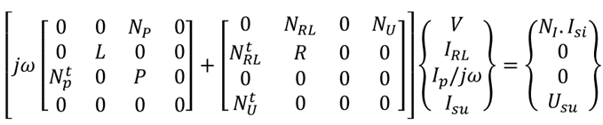
- Generic solver
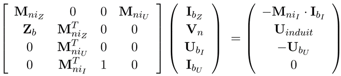
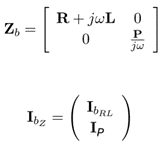
With the M and N are partial incidence matrices related to the dual mesh. We can see that the relationship between matrix P (representing the parasitic capacitance values) and IP (representing current through parasitic capacitance) is written differently. For the state solver, 1/jω is written in the vector of unknowns, while for the generic solver it is written in the matrix. This is why state solvers converge more quickly
Solver preconditioning parameters
- Preconditioner type: for this option, three variants
are possible
- Without: there is no preconditioner.
- LU_MUMPS: the Mumps solver is used to perform the LU decomposition of a specific preconditioning matrix. Then the decomposed matrix is applied to the iterative solver at each iteration.
- Diagonal: for the linear system A . x = b, the diagonal of the matrix A is used as a preconditioner.