Fatigue using S-N (Stress - Life) Method
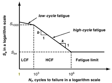
OptiStruct uses the S-N approach for calculating the fatigue life. The S-N approach is suitable for high cycle fatigue, where the material is subject to cyclical stresses that are predominantly within the elastic range. Structures under such stress ranges should typically survive more than 1000 cycles.
Since S-N theory deals with uniaxial stress, the stress components need to be resolved into one combined value for each calculation point, at each time step, and then used as equivalent nominal stress applied on the S-N curve.
- Fatigue Material Properties (S-N Curve)
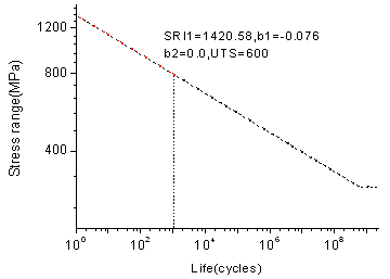
Figure 3. Two Segment S-N Curve 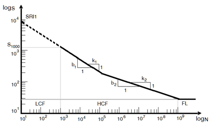
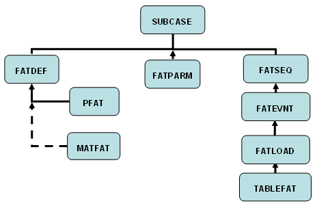
- FATDEF
- Defines the elements and associated fatigue properties that will be used for the fatigue analysis.
- PFAT
- Defines the finish, treatment, layer and the fatigue strength reduction factors for the elements.
- MATFAT
- Defines the material properties for the fatigue analysis. These properties should be obtained from the material's S-N curve (Figure 3). The S-N curve, typically, is obtained from completely reversed bending on mirror polished specimen. S-N curves can be one segment or two segments.
- Fatigue Parameters
Figure 4. Mean Stress Correction 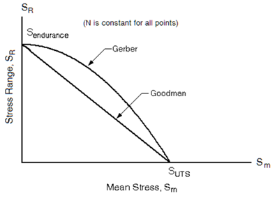
- FATPARM
- Defines the parameters for the fatigue analysis. These include stress combination method, mean stress correction method (Figure 4), Rainflow parameters, Stress Units.
- Fatigue Sequence and Event Definition
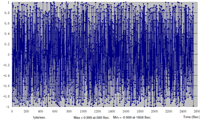
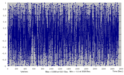
Figure 5. Load Time History 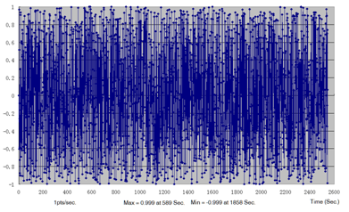
- FATSEQ
- Defines the loading sequence for the fatigue analysis. This card can refer to another FATSEQ card or a FATEVNT card.
- FATEVNT
- Defines loading events for the fatigue analysis.
- FATLOAD
- Defines fatigue loading parameters.
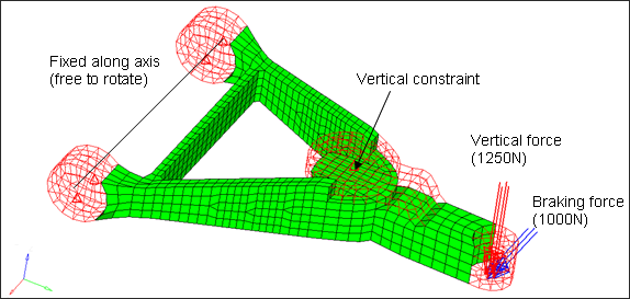
The model being used for this exercise is that of a control arm, as shown in Figure 1. Loads and boundary conditions and two static loadcases have already been defined on this model.
Launch HyperMesh and Set the OptiStruct User Profile
-
Launch HyperMesh.
The User Profile dialog opens.
-
Select OptiStruct and click
OK.
This loads the user profile. It includes the appropriate template, macro menu, and import reader, paring down the functionality of HyperMesh to what is relevant for generating models for OptiStruct.
Import the Model
-
Click .
An Import tab is added to your tab menu.
- For the File type, select OptiStruct.
-
Select the Files icon
 .
A Select OptiStruct file browser opens.
.
A Select OptiStruct file browser opens. - Select the ctrlarm.fem file you saved to your working directory.
- Click Open.
- Click Import, then click Close to close the Import tab.
Set Up the Model
Define TABFAT Load Collector
- Make sure the Utility menu is selected in the View menu. Click .
- Click on the Utility menu beside the Model tab in the browser. In the Tools section, click on TABLE Create.
- Set Options to Import table.
- Set Tables to TABFAT.
- Click Next.
- Browse for the loading file.
- In the Open the XY Data File dialog box, set the Files of type filter to CSV (*.csv).
- Open the load1.csv file you saved to your working directory.
- Create New Table with Name table1.
-
Click Apply to save the table.
The curve table1 with TABFAT card image is created.
- Browse for a second loading file load2.csv.
- Create New Table with Name table2.
-
Click Apply to save the table.
The curve table2 with TABFAT card image is created.
-
Exit from the Import TABFAT window.
Tables appear under Curve in the Model Browser.Note: A file in DAC format can very easily be imported in HyperGraph and converted to CSV format to be read in HyperMesh.
Define TABLOAD Load Collector
- In the Model Browser, right-click and select .
- For Name, enter FATLOAD1.
- Click Color and select a color from the color palette.
- For Card Image, select FATLOAD from the drop-down menu.
- For TID (table ID), select table1 from the list of curves.
- For LCID (load case ID), select SUBCASE1 from the list of load steps.
- Set LDM (load magnitude) to 1.
- Set Scale to 3.0.
- Repeat the process to create another load collector named FATLOAD2 with FATLOAD as card image and pointing to table2 and SUBCASE2.
- Set LDM to 1 and Scale to 3.0.
Define TABEVNT Load Collector
- In the Model Browser, right-click and select .
- For Name, enter FATEVENT.
- For Card Image, select FATEVNT.
- Set FATEVNT_NUM_FLOAD to 2.
-
Click on the Table icon
 next to the
Data field and select FATLOAD1 for
FLOAD(1) and FATLOAD2 for FLOAD(2) in
the pop-out window.
next to the
Data field and select FATLOAD1 for
FLOAD(1) and FATLOAD2 for FLOAD(2) in
the pop-out window.
Define TABSEQ Load Collector
- In the Model Browser, right-click and select .
- For Name, enter FATSEQ.
- For Card Image, select FATSEQ.
-
For FID (Fatigue Event Definition), select FATEVENT from
the list of load collectors.
Defining the sequence of events for the fatigue analysis is completed. The Fatigue parameters are defined next.
Define Fatigue Parameters
- In the Model Browser, right-click and select .
- For Name, enter fatparam.
- For Card Image, select FATPARM.
- Verify TYPE is set to SN.
- Set STRESS COMBINE to SGVON (Signed von Mises).
- Set STRESS CORRECTION to GERBER.
- Set STRESSU to MPA (Stress Units).
- Set RAINFLOW RTYPE to LOAD.
- Set CERTNTY SURVCERT to 0.5.
Define Fatigue Material Properties
The material curve for the fatigue analysis can be defined on the MAT1 card.
-
In the Model Browser, click on the
Aluminum material.
The Entity Editor opens.
- In the Entity Editor, set SN to MATFAT.
- Set UTS (ultimate tensile stress) to 600.
-
For the SN curve set (these values should be obtained from the material's SN
curve):
- SRI1
- 1420.58
- B1
- -0.076
- NC1
- 5.0e8
- SE
- 0.1
Define PFAT Load Collector
- In the Model Browser, right-click and select .
- For Name, enter pfat.
- For Card Image, select PFAT.
- Set LAYER to TOP.
- Set FINISH to NONE.
- Set TRTMENT to NONE.
Define FATDEF Load Collector
- In the Model Browser, right-click and select .
- For Name, enter fatdef.
- For Card Image, select FATDEF.
- Select the PTYPE check box, then select the PSHELL check box.
- Select shell for PID, and pfat for PFATID in the pop-up window.
Define the Fatigue Load Step
- In the Model Browser, right-click and select .
- For Name, enter Fatigue.
- Set the Analysis type to fatigue.
- For FATDEF, select fatdef.
- For FATPARM, select fatparam.
- For FATSEQ, select fatseq.
Submit the Job
-
From the Analysis page, click the OptiStruct
panel.
Figure 10. Accessing the OptiStruct Panel 
- Click save as.
-
In the Save As dialog, specify location to write the
OptiStruct model file and enter
ctrlarm_hm for filename.
For OptiStruct input decks, .fem is the recommended extension.
-
Click Save.
The input file field displays the filename and location specified in the Save As dialog.
- Set the export options toggle to all.
- Set the run options toggle to analysis.
- Set the memory options toggle to memory default.
- Click OptiStruct to launch the OptiStruct job.
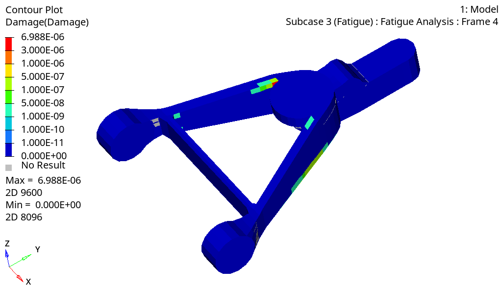
Review the Results
- When the analysis process completes, click HyperView to launch the results.
- In the Results tab, select Subcase 3 (Fatigue) from the subcase field.
-
On the Results toolbar, click
 to open the
Contour panel.
to open the
Contour panel.
-
Set Result type to Damage and click
Apply to contour the elements.
Figure 11. Elemental Damage Results