OS-T: 1330 Acoustic Analysis of a Half Car Model
The purpose of this tutorial is to evaluate the vibration characteristics of a half car model subjected to Fluid - Structure interaction. The fluid that is being referred to is air. Essentially, the noise level or the sound level is evaluated inside the car at a location near the ear of the driver which is the main response location inside the fluid.
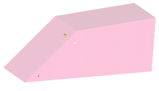
The half car model is excited at the bottom of the car, as shown by a red constraint symbol (triangle) in Figure 1. The excitation provided is with the application of a unit load along the direction of the height of the car (Z-axis).
Launch HyperMesh and Set the OptiStruct User Profile
-
Launch HyperMesh.
The User Profile dialog opens.
-
Select OptiStruct and click
OK.
This loads the user profile. It includes the appropriate template, macro menu, and import reader, paring down the functionality of HyperMesh to what is relevant for generating models for OptiStruct.
Open the Model
- Click .
- Select the Half_Car.hm file you saved to your working directory.
-
Click Open.
The Half_Car.hm database is loaded into the current HyperMesh session, replacing any existing data.
Set Up the Model
Create Materials and Properties and Assign to Structural and Fluid Elements
- In the Model Browser, right-click and select .
- For Name, enter MAT1_shells.
- For Card Image, select MAT1 from the drop-down menu.
-
Fill in the fields for E, Nu and Rho, respectively as
2.1e04, 0.33 and
8.0e-10.
Figure 2. 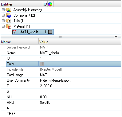
- In the Model Browser, right-click and select .
- For Name, enter MAT10_Solids.
- For Card Image, select MAT10 from the drop-down list.
- Fill in the fields for Rho and C respectively as 1.2e-13 and 3.4e5.
- In the Model Browser, right-click and select .
- For Name, enter Shells.
- For Card Image, select PSHELL from the drop-down menu.
- For Material, click .
- In the Select Material dialog, select MAT1_shells from the list of materials and click OK to complete the selection.
- Enter the thickness for the shell component by clicking T, and entering 2.0.
- In the Model Browser, right-click and select .
- For Name, enter Solids.
- For Card Image, select PSOLID from the drop-down menu.
- For Material, click .
- In the Select Material dialog, select MAT10_Solids.
- For FCTN, select PFLUID.
-
Click on the fluid component.
The component entry is displayed in the Entity Editor.
- For Property, click .
- In the Select Property dialog, select the property solids.
-
Click on the structure component.
The component entry is displayed in the Entity Editor.
- For Property, click .
- In the Select Property dialog, select the property shells.
Create Load Collectors
In this step the model is unconstrained and a unit vertical load is applied acting upwards in the positive z-direction at a point on the base of the car (shown in page 1). The model can be unconstrained as the solver applies PARAM, INREL -2 by default to avoid the model from experiencing a rigid body motion.
-
In the Model Browser, right-click and select from the context menu.
A default load collector displays in the Entity Editor.
- For Name, enter unit-load.
- Click Color and select a color from the color palette.
- Set Card Image to None and click Close.
-
Verify unit_load is the current load collector. If it is not the current load
collector, right-click on unit_load in the Model Browser and select Make Current from
the context menu.
Figure 3. 
Tip: In the Model Browser, Load Collectors folder, the current load collector is bold. - Click .
Create a Unit Load at a Point
- From the Analysis page, click constraints.
- Select the create subpanel using the radio buttons on the left-hand side of the panel.
- Select node number 19072 on the car model by clicking nodes >> by id.
- Uncheck all dofs, except dof3.
- Click the = to the right of dof3 and enter a value of 1.
- For Load Types =, select DAREA from the extended entity selection menu.
-
Click create.
This applies a unit load to the selected node.
Figure 4. 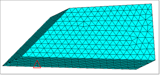
- Click return.
Create a Frequency Range Table
-
In the Model Browser, right-click and
select .
A new window opens.
- For Name, enter tabled1.
- In the table, enter x(1) = 0.0, y(1) = 1.0, x(2) = 200, y(2) = 1.0.
- Close the Curve Editor window.
- From Curves, select tabled1.
- Click Color and select from the palette.
-
For Card
Image, select TABLED1
from the drop-down menu.
This provides a frequency range of 0.0 to 200 with a constant 1.0 over this range.
Figure 5. 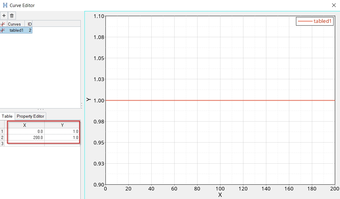
Create a Frequency Dependent Dynamic Load
- In the Model Browser, right-click and select .
- For Name, enter rload1.
- For Config type, select Dynamic Load – Frequency Dependent from the drop-down menu.
- For Type, select RLOAD1 from the drop-down menu.
- For EXCITEID, click .
- In the Select Loadcol dialog, select unit-load from the list of load collectors and click OK to complete the selection.
-
For the TC field, select the curve tabled1.
The type of excitation can be an applied load (force or moment), an enforced displacement, velocity, or acceleration. The field TYPE in the RLOAD1 load step input defines the type of load. The type is set to applied load by default.
A typical RLOAD1 card appears, as shown below.Figure 6. 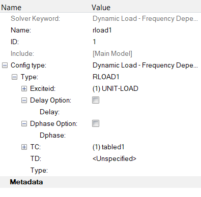
- In the Model Browser, right-click and select .
- For Name, enter freq1.
- Click Color and select a color from the color palette.
- For Card Image, select FREQi from the drop-down menu.
- Check the box next to FREQ1.
- For NUMBER_OF_FREQ1, enter a value of 1, press Enter.
-
Click
 next to the Data field and enter, F1= 0.0, DF=
1.0, and NDF= 200.
This provides a set of frequencies beginning with 0.0, incremented by 1.0 and 200 frequencies increments and the card appears as shown below on the GUI.
next to the Data field and enter, F1= 0.0, DF=
1.0, and NDF= 200.
This provides a set of frequencies beginning with 0.0, incremented by 1.0 and 200 frequencies increments and the card appears as shown below on the GUI.Figure 7. 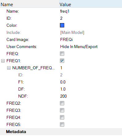
- In the Model Browser, right-click and select .
- For Name, enter eigrl1.
- Click Color and select a color from the color palette.
- For Card Image, select EIGRL from the drop-down menu.
- For V2, enter a value of 600.0.
-
For ND, enter a value of 50.
This specifies a range of frequency between an initial frequency and 600 Hz for eigenvalue extraction using the Lanczos method.
-
Similarly, follow steps 8.1 to 8.6 to create another load collector named
eigrl2.
Figure 8. 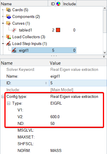
- In the Model Browser, right-click and select .
- For Name, enter subcase1.
- Click Color and select a color from the color palette.
- For Analysis type, select Freq.resp (modal) from the drop-down menu.
- For METHOD(STRUCT), select eigrl1 from the list of load collectors.
- For METHOD(FLUID), select eigrl2 from the list of load collectors.
- For DLOAD, select rload1 from the list of load collectors.
-
For FREQ, select freq1 from the list of load
collectors.
An OptiStruct subcase has been created which references the constraints, the unit load in the load collector rload1 with a set of frequencies defined in load collector freq1 and modal method defined in the load collector eigrl.
- In the Model Browser, right-click and select .
- For Name, enter SETA.
- For Card Image, select None from the drop-down menu.
- Leave the Set Type switch set to non-ordered type.
- For Entity IDs, click the yellow Nodes panel and select nodes with ID 18881.
- Click proceed.
Create a Set of Frequencies
- In the Model Browser, right-click and select .
- For Name, enter freq1.
- Click Color and select a color from the color palette.
- For Card Image, select FREQi from the drop-down menu.
- Check the FREQ1 option and enter 1 in the NUMBER_OF_FREQ1 field.
-
Update the following fields in the pop-out window.
- For F1, enter 0.0.
- For DF, enter 1.0.
- For NDF, enter 200.
-
Click Close.
This provides a set of frequencies beginning with 0.0, incremented by 1.0 and 200 frequencies increments and the card appears as shown below on the GUI.
Create the Modal Method for Eigenvalue Analysis
- In the Model Browser, right-click and select .
- For Name, enter eigrl1.
- For Config type, select Real Eigen Value Extraction.
- For Type, select EIGRL from the drop-down menu.
- For V2, enter a value of 600.0.
-
For ND, enter a value of 50.
This specifies a range of frequency between an initial frequency and 600 Hz for eigenvalue extraction using the Lanczos method.
-
Similarly, create another load step input named eigrl2.
Figure 9.
Create a Load Step
-
In the Model Browser, right-click and
select .
A default load step template is now displayed in the Entity Editor below the Model Browser.
- For Name, enter subcase1.
- For Analysis type, select Freq.resp (modal) from the drop-down menu.
- For METHOD(STRUCT), select eigrl1.
- For METHOD(FLUID), select eigrl2 from the list of load step inputs.
- For DLOAD, select rload1 from the Select Load Step Inputs pop-out window.
- For FREQ, click
-
From the Select Loadcol dialog, select
freq1.
An OptiStruct subcase has been created which references the constraints, the unit load in the load step input rload1 with a set of frequencies defined in load collector freq1 and modal method defined in the load step input eigrl.
Create a Set of Nodes
- In the Model Browser, right-click and select .
- For Name, enter SETA.
- For Card Image, select SET_GRID.
- Leave the Set Type switch set to non-ordered type.
- For Entity IDs, select Nodes from the selection switch.
- Click Nodes and select nodes 18881.
- Click proceed.
Create a Set of Outputs
- From the Analysis page, click control cards.
-
Click on ACMODL.
This defines the model parameters for fluid-structure interface.
- Click [INTER] and select DIFF.
- Click [INFOR] and select ALL.
- Click return to exit this menu.
-
Select GLOBAL_OUTPUT_REQUEST. Then check the box to the
left of DISPLACEMENT.
A new window appears in the work area screen.
- Click the field box FORM and select PHASE from the pop-up menu.
-
Click the field box OPTION and select
SID from the pop-up menu.
A new field appears in yellow.
-
Double-click the yellow SID box and select
SETA from the pop-up selection on the bottom left
corner.
A value of 1 now appears below the SID field box. This sets the output for only the nodes in set 1.
- Click return to exit this menu.
- Select GLOBAL_CASE_CONTROL.
- Check the box next to FREQ.
- Click FREQ and select the load collector freq1.
- Click return to exit this menu and click next.
-
Select the OUTPUT subpanel.
A new window appears in the work area.
- Specify number of outputs = 4.
- Verify KEYWORD is set to HGFREQ.Using HGFREQ results in a frequency output presentation for HyperGraph.
-
Double-click on the box beneath FREQ and select ALL from
the pop-up selection.
Choosing ALL outputs results for all frequencies.
- Verify KEYWORD is set to OPTI.
- Double-click on the box beneath FREQ and select ALL from the pop-up selection.
- Similarly under KEYWORD select PUNCH and H3D.
- Click return to exit this menu.
- Select PARAM.
- Click AUTOSPC.
-
Scroll down and check the box next to G.
A new window appears in the work area screen.
-
Click below G_V1, and input a value of 0.06 into the
field box.
This value specifies a uniform structural damping coefficient and is obtained by multiplying the critical damping [ ] ratio by 2.0.
- Check the box next to GFL.
- Click below [VALUE] and enter 0.12.
- Click return to exit the PARAM menu.
- Click return to exit the control cards menu.
Submit the Job
-
From the Analysis page, click the OptiStruct
panel.
Figure 10. Accessing the OptiStruct Panel 
- Click save as.
-
In the Save As dialog, specify location to write the
OptiStruct model file and enter
Half_car for filename.
For OptiStruct input decks, .fem is the recommended extension.
-
Click Save.
The input file field displays the filename and location specified in the Save As dialog.
- Set the export options toggle to all.
- Set the run options toggle to analysis.
- Set the memory options toggle to memory default.
- Click OptiStruct to launch the OptiStruct job.
- Half_car.html
- HTML report of the analysis, providing a summary of the problem formulation and the analysis results.
- Half_car.out
- OptiStruct output file containing specific information on the file setup, the setup of your optimization problem, estimates for the amount of RAM and disk space required for the run, information for each of the optimization iterations, and compute time information. Review this file for warnings and errors.
- Half_car.h3d
- HyperView binary results file.
- Half_car.res
- HyperMesh binary results file.
- Half_car.stat
- Summary, providing CPU information for each step during analysis process.
Review the Results
-
From the OptiStruct panel, click HyperView.
HyperView is launched and the results are loaded. A message window appears to inform of the successful model and result files loading into HyperView.
- Click Close to close the message window, if one appears.
-
In the HyperView window, click .
An Open Session File window opens.
- Select the directory where the job was run and select the file Half_car_freq.mvw.
-
Click Open.
A discard warning appears.
-
Click Yes.
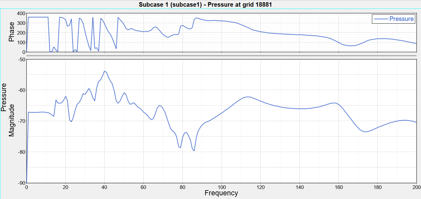
Two graphs per page and a total of one page are displayed in HyperGraph. The graph title shows Subcase 1 (subcase 1) pressure at grid 18881.
-
Click the Axis toolbar icon
 .
.
- Make sure the Axis is set to Primary and Horizontal.
- Click the Scale and Tics tab.
-
Make sure the toggle is set to Linear.
Figure 11. 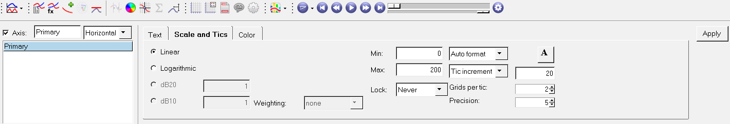
- In the Axis, toggle from Horizontal to Vertical.
- Click on the Scale and Tics (Magnitude) tab.
-
Make sure the toggle is set to dB10.
Figure 12. 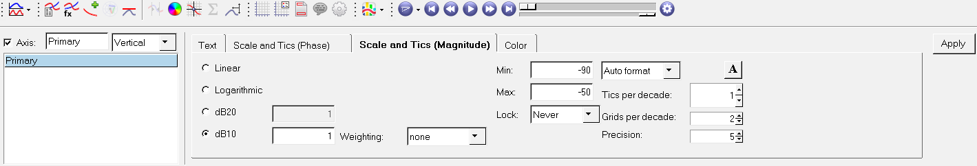
There are two sets of results on this page. The top graph shows Phase Angle verses Frequency (log). The bottom graph shows Magnitude verses Frequency (log) (see figure below) for Pressure at grid 18881.Figure 13.