OS-T: 1315 Modal Transient Dynamic Analysis of a Bracket

In this tutorial, an existing finite element model of a bracket is used to demonstrate how to perform modal transient dynamic analysis using OptiStruct. HyperGraph is used to post-process the deformation characteristics of the bracket under the transient dynamic loads.

Before you begin, copy the file(s) used in this tutorial to your working directory.

bracket_transient.hm

rd2030_pic1 — Figure 1. Finite Element Model of the Bracket

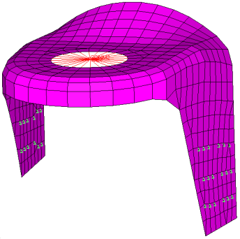
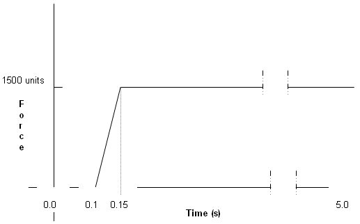
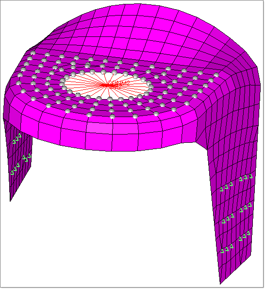
The bracket is constrained at the bottom of the two legs. Transient dynamic loads are to be applied at the grid points of the top, flat surface of the bracket around the hole in the negative z-direction. The time history of the loading is shown in Figure 2. The modal transient analysis is run for a total time of 4 seconds with the time being divided into 800 increments (that is time step is 0.005). Modal damping has been defined as 2% critical damping for all the modes. Modes up to 1000 Hz have been considered. A concentrated mass element is defined at the center of the spider and z-displacements are monitored at the concentrated mass at the center of this hole.

time_history — Figure 2. Time History of Applied Loading

Launch HyperMesh and Set the OptiStruct User Profile

Launch HyperMesh.
The User Profile dialog opens.
Select OptiStruct and click OK.
This loads the user profile. It includes the appropriate template, macro menu, and import reader, paring down the functionality of HyperMesh to what is relevant for generating models for OptiStruct.

Open the Model

Click File > Open > Model.
Select the bracket_transient.hm file you saved to your working directory.
Click Open.
The bracket_transient.hm database is loaded into the current HyperMesh session, replacing any existing data.

Set Up the Model

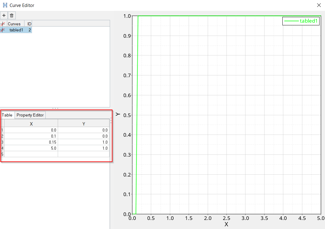
Create a TABLED1 Curve

In the Model Browser, right-click and select Create > Curve.
For Name, enter tabled1.
In the Curve Editor window, enter the values shown in Figure 3.

Figure 3. Table Showing Time History of Loading
Close the Curve Editor.
In Curves, select tabled1.
Click Color and select a color from the color palette.
For Card Image, select TABLED1 from the drop-down menu.
The curve TABLED1 that defines the time history of the loading has been created.

Create TSTEP Load Collector

In the Model Browser, right-click and select Create > Load Collector.
For Name, enter tstep.

Transient time step to define the time step intervals at which solution is generated and output.
Click Color and select a color from the color palette.
For Card Image, select TSTEP from the drop-down menu.
For TSTEP_NUM, enter 1 and press Enter.
For N, enter the number of time steps as 800.
For DT, enter the time increment of 0.005.
The total time applied to the load is: 800 x 0.005 = 4 seconds. This is the time step at which output is requested. NO has a default value of 1.0.
Click Close.

Create a DAREA Load Collector

To define forces on the top surface of the bracket.

In the Model Browser, right-click and select Create > Load Collector.
For Name, enter darea.
Click Color and select a color from the color palette.
For Card Image, select NONE.
Click BCs > Create > Constraints to open the Constraints panel.
Click nodes > by sets.
Two sets are displayed.
Select force and click select.
The nodes that belong to the set force get selected.
Figure 4.
Uncheck all degrees of freedom (dof), except dof3 by clicking the box next to each, indicating that dof3 is the only active degree of freedom.
For dof3, enter a value of -1500.
For load types=, select DAREA.
Click create.
This creates a force of 1500 units applied to the selected nodes in the negative z direction.
Click return to go back to the main menu.

Create a TABDMP1 Curve

The modal damping table to define damping as a tabular function of frequency.

In the Model Browser, right-click and select Create > Curve.
For Name, enter tabdmp1.
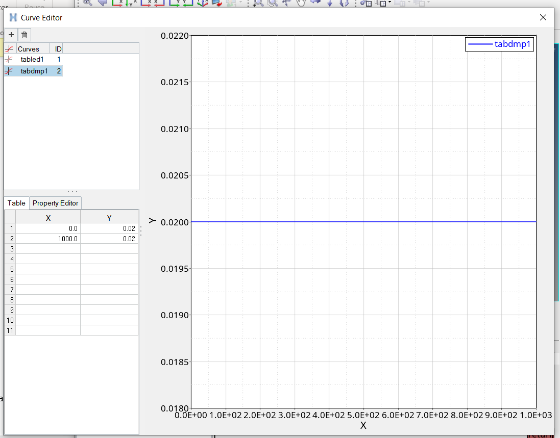
In the Curve Editor window, enter the values shown in Figure 5.

Figure 5.
Close the Curve Editor.
In Curves, select tabdmp1.
Click Color and select a color from the color palette.
For Card Image, select TABDMP1 from the drop-down list.
For TYPE, switch to CRIT to specify critical damping.
Populate the frequency and damping values for frequencies 0 and 1000 Hz and damping to be 0.02. This provides a table of damping values for the frequency range of interest.

Apply Concentrated Mass

Select the 1D panel radio button.
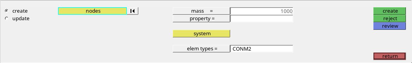
On the panel, select masses.
Select nodes > by id.
In the dialog, enter 395 for the node ID.
For mass, enter 1000.

Figure 6.
Click create and then click return.

Create a EIGRL Load Step Input

In the Model Browser, right-click and select Create > Load Step Inputs.
For Name, enter eigrl.
Click Color and select a color from the color palette.
For Config type, select Real Eigen value extraction from the drop-down menu.
For Type, select EIGRL from the drop-down menu.
For V1, enter 0.0.
For V2, enter 1000.0.
Leave the ND field blank to extract modes up to 1000 Hz.

Create a TLOAD1 Load Step Input

In the Model Browser, right-click and select Create > Load Step Inputs.
For Name, enter tload1.
For Config type, select Dynamic Load – Time Dependent from the drop-down list.
Click Color and select a color from the color palette.
For Type, select TLOAD1 from the drop-down list.
For Exciteid, click Unspecified > Loadcol.
In the Select Loadcol dialog, select darea from the list of load collectors (created in the last section to define the forces on the top surface of the bracket).
Click OK to complete the selection.
Similarly select the tabled1 curves for the TID field (to define the time history of the loading).
The type of excitation can be an applied load (force or moment), an enforced displacement, velocity, or acceleration. The field [TYPE] in the TLOAD1 load step inputs, defines the type of load. The type is set to applied load by default.

Create a Load Step

To perform the modal transient dynamic analysis.

In the Model Browser, right-click and select Create > Load Step from the context menu.
For Name, enter transient.
Set Analysis type type to Transient (modal).
For SPC, select spc.
For DLOAD, select tload1.
For TSTEP(TIME), select tstep.
For METHOD (STRUCT), select the load step input eigrl.
For SDAMPING (STRUCT, select the Curve tabdmp1.

A subcase is created that specifies the loads, boundary conditions, and damping for modal transient dynamic analysis.

Create Output Requests

From the Analysis page, click control cards.
In the Card Image dialog, click GLOBAL_OUTPUT_REQUEST.
Define the DISPLACEMENT card.
1. Select DISPLACEMENT.
2. Leave the field for FORMAT(1) blank.
3. For FORM(1), select BOTH.
4. For OPTION(1), select SID.
5. Double-click the SID selector and select center.
6. Click return.
The center set represents the node at the center of the spider attached to the mass element, which is node 395.
Define the OUTPUT card.
1. Select OUTPUT.
2. In the number_of_outputs= field, enter 2.
3. For KEYWORD, select H3D and HGTRANS.
4. For FREQ, select ALL for both.
5. For H3D KEYWORD, set the other field to blank.
6. Click return.
Click return to exit from the dialog.

Submit the Job

From the Analysis page, click the OptiStruct panel.

Figure 7. Accessing the OptiStruct Panel
Click save as.
In the Save As dialog, specify location to write the OptiStruct model file and enter bracket_transient_modal for filename.
For OptiStruct input decks, .fem is the recommended extension.
Click Save.
The input file field displays the filename and location specified in the Save As dialog.
Set the export options toggle to all.
Set the run options toggle to analysis.
Set the memory options toggle to memory default.
Click OptiStruct to launch the OptiStruct job.

If the job is successful, new results files should be in the directory where the bracket_transient_modal.fem was written. The bracket_transient_modal.out file is a good place to look for error messages that could help debug the input deck if any errors are present.

The default files written to the directory are:

bracket_transient_modal.html: HTML report of the analysis, providing a summary of the problem formulation and the analysis results.
bracket_transient_modal.out: OptiStruct output file containing specific information on the file setup, the setup of your optimization problem, estimates for the amount of RAM and disk space required for the run, information for each of the optimization iterations, and compute time information. Review this file for warnings and errors.
bracket_transient_modal.h3d: HyperView binary results file.
bracket_transient_modal.res: HyperMesh binary results file.
bracket_transient_modal.stat: Summary, providing CPU information for each step during analysis process.
bracket_transient_modal.mvw: HyperView session file.; This file is only created when transient analysis is performed. This file automatically creates plots for the displacement, velocity and acceleration results contained in the file.

View the Results

From the OptiStruct panel, click HyperView to launch HyperView.
From the menu bar, click File > Open > Session.
In the Open Session File dialog, open bracket_transient_modal_tran.mvw from the directory in which the input file was run.
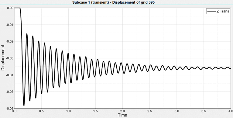
Since the loading is applied only in the z-direction, you are interested in the z-displacement time history of node 395.

Plots for the displacement results contained in the file are created.
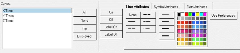
On the Visualization toolbar, click to open the Curves Attributes panel.
Under Curves, individually select the X Trans and Y Trans curves and click Off.

Figure 8.

The X Trans and Y Trans curves are turned off.
Click to fit the y-axis (that is Z displacement) of node 395.
If desired, you can change the color and/or line attributes of the curve.

As can be observed from the above image, the displacements of node 395 are in the negative z-direction as the loading is in the -z direction too. The displacements eventually damp out due to the structural damping present in the model.

rd2030_pic7 — Figure 9. Z-displacement time history of the concentrated mass. at center of spider for direct transient dynamic analysis