OS-T: 1390 Pretensioned Bolt Analysis of an IC Engine Cylinder
Head, Gasket and Engine Block System
This tutorial outlines the procedure to perform both 1D and 3D pretensioned bolt
analysis on a section of an IC Engine. The pretensioned analysis is conducted to measure the
response of a system consisting of the cylinder head, gasket and engine block connected by
four head bolts subjected to a pretension force of 4500 N each.
Before you begin, copy the file(s) used in this tutorial to your
working directory.
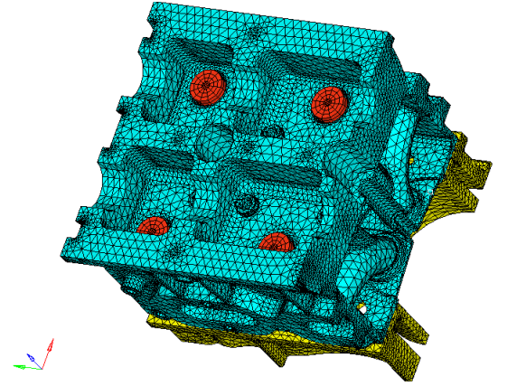
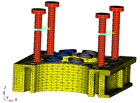
Figure 1. Model Showing the Cylinder Head, Engine Block and Head
Bolts
The model consists of eight predefined components along with their corresponding
property and material allocations. A contact surface (PT_Surf) has been defined,
which is used for 3D pretensioning of an existing pretension surface. The pretension
sections for 1D pretensioning have also been created on two of the four bolts and
the sectioned bolts are reconnected using 1D beam elements (via rigids). A
predefined visualization aid is also available under View,
which allows you to easily look at the pretensioned sections of the four bolts.
Contact surfaces and Contact Interfaces
(TYPE=FREEZE) between the various parts have
also been created so you can focus on the Pretensioning aspect of the tutorial.
Pretensioned Bolt Analysis
Many engineering assemblies are put together using bolts, which are usually
pretensioned before application of working loads. A typical sequence is
described below. For further detailed information, refer to Pretensioned Bolt Analysis in the User
Guide.
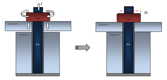
In Step 1, upon preliminary assembly of the structure, the
nuts on respective bolts are tightened, usually by applying prescribed torque
(which translates into prescribed tension force according to the pitch of the
thread).
As a result, the working part of the bolt becomes shorter by a
distance . This distance depends upon the applied force,
the compliance of the bolt and of the assembly being pretensioned.Figure 2. Step 1 of Pretensioned Assembly. Application of Pretensioning Loads
From the perspective of FEA analysis, it is important to recognize
that:
Pretensioning actually shortens the working part of the bolt by removing
a certain length of the bolt from the active structure (in reality this
segment slides through the nut, yet the net effect is the shortening of
the working length of the bolt). At the same time the bolt stretches,
since now the smaller effective length of the bolt material has to span
the distance from the bolt mount to the nut.
Calculation of each bolt's shortening , due to applied forces F, requires FEA
solution of the entire model with the pretensioning forces applied. This
is because the amount of nut movement, due to given force depends on the
compliance of the bolts, of the assembly being bolted and is also
affected by cross-interaction between multiple bolts being pretensioned.
At the end of Step 1, the amount of shortening for each bolt is established and "locked",
simply by leaving the nuts at the position that they reached during the
pretensioning step.
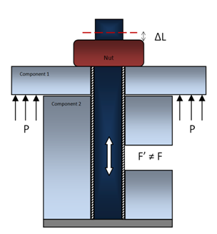
In Step 2, with the shortening of all the bolts "locked", other loads are
applied to the assembly. At this stage the stresses and strains in the bolts
will usually change, while the length of material removed remains constant for each bolt.Figure 3. Step 2 of Pretensioned Assembly. Application of Working Loads with 'Locked' Bolt Shortening
Launch HyperMesh and Set the OptiStruct User Profile
Launch HyperMesh.
The User Profile dialog opens.
Select OptiStruct and click
OK.
This loads the user profile. It includes the appropriate template, macro
menu, and import reader, paring down the functionality of HyperMesh to what is relevant for generating models for
OptiStruct.
Open the Model
Click File > Open > Model.
Select the Pretension.hm file you saved to
your working directory.
Click Open.
The Pretension.hm database is loaded
into the current HyperMesh session, replacing any
existing data.
Set Up the Model
This tutorial helps the you apply 1D and 3D bolt pretensioning to the four head bolts
(two of each) and then apply a pressure load to the constrained system. The applied
pressure load models the pressure on the inside walls of an IC engine due to
combustion. Pressure within the engine compartment varies with time (transient);
however, you capture the response of the system at a specific instant frozen in
time. A constant single-valued pressure load of 1 Pascal is applied to the inner
walls of the cylinder head and the engine block.
Gasket behavior is nonlinear and it may undergo cycles of loading and unloading which
lead to changes in its properties at each step. In this tutorial, which focuses on
1D and 3D pretensioning, the loading and unloading paths for the gasket material are
pre-populated in the MGASK Data Entry via the
TABLES# entries referenced by corresponding load collectors.
As the nonlinear static analysis is running, the initial applied pressure load is
compared with corresponding values within the loading/unloading path tables and the
initial material properties of the gasket are determined. The nonlinear properties
of the gasket via the MGASK Data Entry are a function of pressure
and the closure distance (Refer to MGASK Bulk Data Entry for more
information). FREEZE contact has been predefined for all parts in
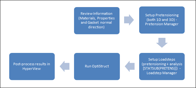
contact.Figure 4. Tutorial Process Flow
Review Material Properties
The imported model contains a large amount of pre-populated information which
allows us to focus on the pretensioning section in this tutorial. As previously
explained, all material and properties are predefined for the gasket, engine block,
cylinder head and head bolts. The material properties of steel are assigned to all
components except the gasket.
In the Model Browser, right-click and select
Expand All.
Click on STEEL in the Model Browser
under Material.
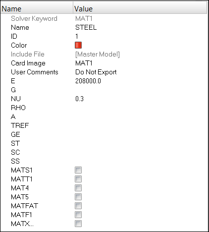
The MAT1 entry is displayed in the Entity Editor with pre-populated field values.
Make sure that the values on the MAT1 Bulk Data Entry for
the material properties of steel are input as shown below.
Figure 5. Reviewing the Material - Steel
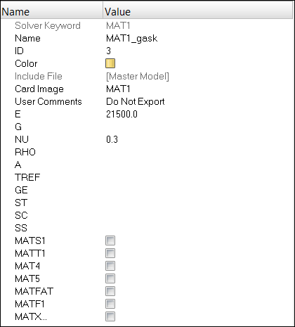
Select MAT1_gask in the Model Browser.
Make sure that the values on the MAT1 Bulk Data Entry for
the material properties of the gasket are input as shown below.
Figure 6. Reviewing the Material - Gasket
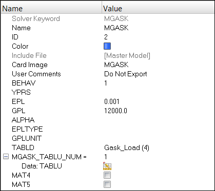
Click on MGASK.
Make sure that the values on the MGASK Bulk Data Entry for
the material properties of the gasket are input as shown below.
Figure 7. Reviewing the Nonlinear Gasket Material Properties - MGASK
Tip: The TABLD and TABLU(1) fields (Gasket loading and unloading
paths) in Figure 7 are defined by TABLES1 Bulk Data Entries in separate
curves named Gask_Load and Gask_Unload1, respectively.
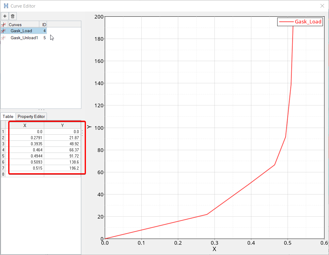
Click on Gask_Load in the Curves folder and then
right-click and select Edit to view the data.
Make sure that the values on the TABLES1 Bulk Data Entry
defining the gasket loading paths are input as shown below.
Figure 8. Reviewing the Gasket Loading Paths - TABLES1
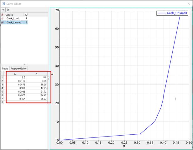
Similarly, make sure that the values on the TABLES1 Bulk
Data Entry defining the gasket unloading paths (curves Gask_Unload1) are input
as shown below.
Figure 9. Reviewing the Gasket Unloading Paths - TABLES1
Tip: You can review, in a similar manner, the remaining predefined
data entries like properties and load collectors. The procedure for load
collector review is not as straight forward, as shown above in some cases;
however, this has been thoroughly illustrated in various other tutorials for
your benefit.
The gasket normal direction is now reviewed by clicking on
normals in the Tools panel.
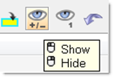
To select the gasket component, use the Show/Hide tool (Figure 10 ) to hide the cylinder head thereby exposing the gasket to view.
Figure 10. Masking (Show/Hide) Tool
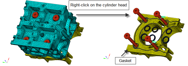
Click on the Show/Hide icon, and right-click on the
cylinder head to hide it from view.
The gasket should now be visible.Figure 11. Exposing the Gasket Component to View Using the Masking Tool
In a similar fashion, hide (right-click) the engine block from view to be able to better visualize the gasket normals.
Click the Show/Hide icon again to deselect it and select
the gasket directly from the modeling window and click
display normals.
The gasket normals can be seen in the modeling window, as shown in Figure 12. Notice that all the normals point in the negative Z direction.Figure 12. Selecting the Gasket Component Figure 13. Displaying the Gasket Normals (Negative Z Direction)
This concludes the review section of the tutorial. You will now focus on generating
contact interfaces, contact surfaces and applying pretensioning to the head
bolts.
Apply 1D and 3D Bolt Pretensioning
Bolt pretensioning analysis determines the response of a system which contains bolts
holding two or more components together as a result of pretensioning. In OptiStruct, pretensioning is applied in an earlier subcase and it
is subsequently referenced to in the subcase where its effect is sought
(STATSUB(PRETENS)).
In the Model Browser, right-click on
Component and select Show from
the context menu.
Hide the CYLINDER_HEAD component by clicking the
Elements icon next to it in the Model Browser.
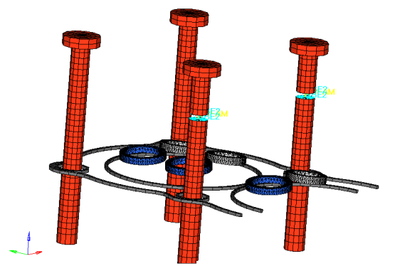
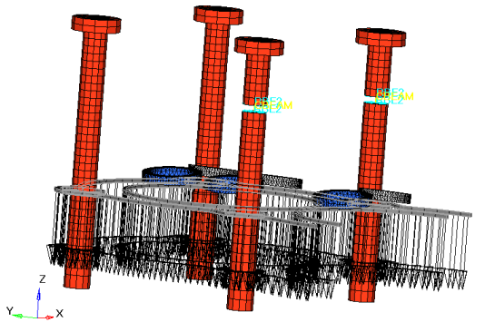
Tip: View1, A predefined visualization option, is included with this
model under View in the Model Browser. Click on the
monitor shaped icon next to View1; this loads a predefined view in the
Model Browser allowing you to view all four bolts in
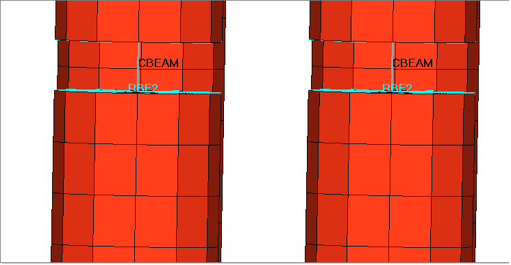
the Y-Z plane. Two bolts have disc-shaped sections cut-off along its length.
These bolts are then reconnected using 1D beam elements
(CBEAM) and two rigid spiders
(RBE2) per bolt. 1D pretensioning can now be applied
to these two bolts. 3D pretensioning requires the creation of a surface at
which pretensioning forces can be applied.
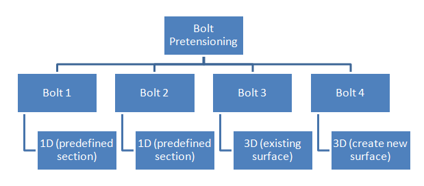
Figure 14. Using the predefined visualization option View1 A surface PT_Surf has been predefined to demonstrate 3D pretensioning on
existing surfaces. To additionally demonstrate 3D pretensioning by creating a
new surface, the fourth bolt is left unchanged.Figure 15. Bolt Pretensioning for this Tutorial Model
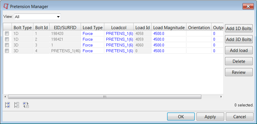
From the menu bar, click Tools > Pretension Manager to access the Pretension Manager.
Click on Add 1D Bolts and select the two 1D beam
elements in bolts 1 and 2 (Figure 18).
Tip: Care must be taken not to use Ctrl+left
mouse click while zooming in and positioning the elements in the graphics
area for selection. Using Ctrl+left mouse click can
lead to the model being rotated about an axis and thus disengaging from the
Y-Z plane of View1. It is recommended to only use Ctrl+right mouse click (dragging action) while working in View1.
Figure 16. Selecting the Predefined 1D Elements for Pretensioning
Select both fields under the Load Type column in the Pretension Manager window
(Click on the first field and then while holding down the Ctrl key, click on the second field). Click on the downward
facing arrow next to the second field and select Force
from the drop-down menu.
In a similar fashion, enter 4500.0 for both bolts in the
Load Magnitude column.
Click Apply.
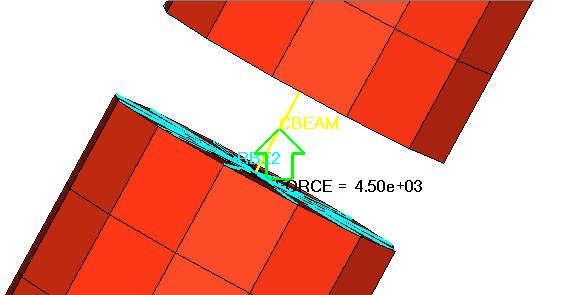
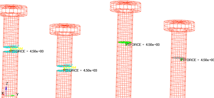
A pretensioning force of 4500.0 N is applied to both 1D bolts, as shown
in Figure 19.Figure 17. Pretensioning Force is Applied to 1D Elements (PTFORCE=4500
N)
Click on Add 3D Bolts and select Select
Existing Surface from the drop-down menu.
Click on the Wireframe elements skin only icon to view
the predefined contact surface PT_Surf on the third bolt.
Tip: If the predefined surface is not visible, then switch on (show)
the PT_Surf entry in the Model Browser by clicking on
the icon next to it.
Click on the displayed predefined surface in the bolt, as shown in Figure 20 and click proceed.
Figure 18. Selecting the Predefined PT_Surf Surface
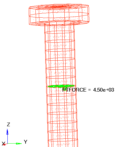
Select Force under the Load Type column and enter
4500.0N for the Load Magnitude column and click
Apply.
A pretensioning force of 4500.0 N is applied normal to the PT_Surf surface, as
shown in Figure 21.Figure 19. Applying a pretensioning force of 4500 N to the predefined surface
PT_Surf on the third bolt
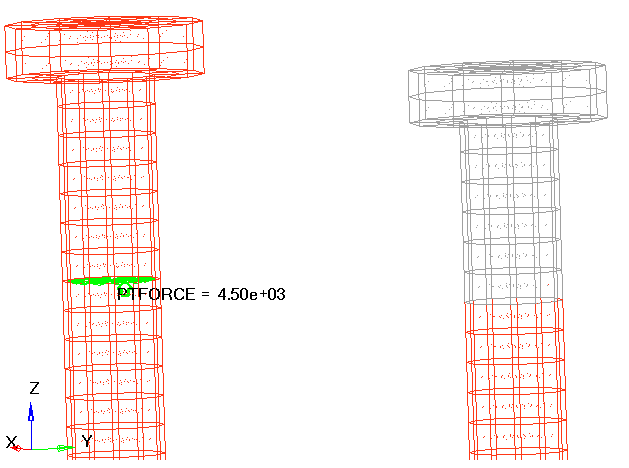
Click on Add 3D Bolts and select Create New
Surface from the drop-down menu.
Toggle 3d faces into elems in the
panel below the graphics area.
Tip: Utilize the click and drag technique (while holding down the
Shift key) described previously to select the
top of the fourth bolt, as shown in Figure 22.
Figure 20. Creating a New Surface for Pretensioning
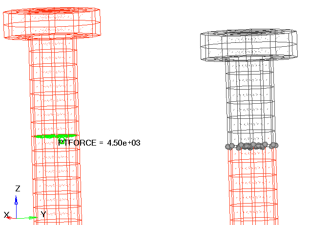
Click on nodes in the panel below the graphics area and
select all the nodes in the surface perpendicular to the Y-Z plane, as shown in
Figure 23.
Tip: The same click and drag technique can be used to select these
nodes (draw a window encompassing the line as the perpendicular surface is a
line in the Y-Z plane).
Figure 21. Selecting the nodes necessary to create a pretensioning
surface
Click create > return to return to the Pretension Manager.
Select Force under the Load Type column and enter
4500.0 N for the Load Magnitude and click
Apply.
Figure 22. Pretension Manager with all Four Pretensioned Bolts
Click OK in the Pretension Manager to view all four
bolts with their respective pretensioning forces, as shown in Figure 25.
Figure 23. Reviewing the Four Pretensioned Bolts
Create a Pretension Loadstep and Subsequent Analysis Loadstep
OptiStruct nonlinear static analysis loadsteps will be
created for both pretensioning and the subsequent analysis. The analysis is nonlinear
due to the presence of contact elements and the gasket loading/unloading paths. The
CNTNLSUB Bulk Data Entry is used to continue the subsequent
nonlinear analysis after pretensioning. Also, the pretensioning subcase is referenced in
the analysis subcase using STATSUB(PRETENS). The Loadsteps Browser will be used to created the loadsteps and assign
respective data entries.
Click on the Shaded Elements and Mesh Lines icon next to the BLOCK and CYLINDER_HEAD components in the
Model Browser to show the hidden components.
Click Tools > Load Step Browser to access the Loadsteps Browser.
Right-click on Loadsteps in the Loadsteps Browser and select New
loadstep.
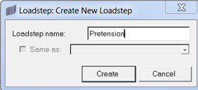
In the Loadstep name: field, enter Pretension and click
Create.
Figure 24. Creating the Pretension Subcase
Select Nonlinear static from the drop-down menu next to
Loadstep type: in the Loadstep Type tab.
Switch to the Load References tab and click on
NLPARM in the list of subcase entries.
Click on Nlparm in the Available nonlinear parameters:
section and then click on the right facing arrow to add it to the selected nonlinear parameter:
section.
Similarly, click on SPC in the Subcase Entry list and
add the Available SPC constraint to the Selected SPC
constraints: section.
Follow the instructions in Steps 6 or 7 to add PRETENS_1
to the list from the PRETENSION Subcase Entry section.
Click OK after all three subcase entries are added to
the Pretension loadstep.
Right-click on Loadsteps in the Loadsteps Browser and select New
loadstep.
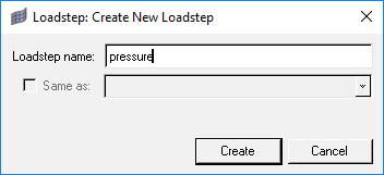
In the Loadstep name: field, enter Pressure and click
Create.
Figure 25. Creating the Pressure Loadstep
Select Nonlinear static from the drop-down menu next to
Loadstep type: in the Loadstep Type tab.
Switch to the Load References tab and click on
NLPARM in the list of subcase entries.
Click on Nlparm in the Available nonlinear parameters:
section and then click on the right facing arrow to add it to the selected nonlinear parameter:
section.
Similarly, click on SPC in the subcase entry list and
add the Available SPC constraint to the Selected SPC
constraints: section.
Follow the instructions in Steps 6 or 7 to add
PRETENSION to the list from the STATSUB(PRETENS)
subcase entry section.
Again, follow the instructions in Steps 6 or 7 to add
PRESSURES to the list from the LOAD subcase entry
section.
Click on the CNTNLSUB subcase entry and check the box
next to CNTNLSUB, additionally select YES from the
pull-down menu next to CNTNLSUB.
Click OK after all five subcase entries are added to the
Pressure loadstep.
Click Close to exit the Loadsteps Browser.
Submit the Job
From the Analysis page, click the OptiStruct
panel.
Figure 26. Accessing the OptiStruct Panel
Click save as.
In the Save As dialog, specify location to write the
OptiStruct model file and enter
Pretension for filename.
For OptiStruct input decks,
.fem is the recommended extension.
Click Save.
The input file field displays the filename and location specified in the
Save As dialog.
Set the export options toggle to all.
Set the run options toggle to analysis.
Set the memory options toggle to memory default.
Click OptiStruct to launch
the OptiStruct job.
If the job is successful, new results files
should be in the directory where the Pretension.fem was written. The Pretension.out file is a good place to look for error messages that could help
debug the input deck if any errors are present.
View the Results
When the message Process completed
successfully is received in the command
window, click HyperView. HyperView is launched and the
results are loaded.
A message window appears to inform of the
successful model and result files loading into
HyperView.
Click Close to close
the message window, if one appears.
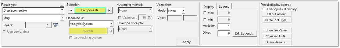
Click the Contour toolbar icon .
Select the first pull-down menu below
Result type: and select
Displacement(v).
Figure 27. Contour plot panel in HyperView
Click Apply, select Subcase 2
(Pressure) from the Results Browser.
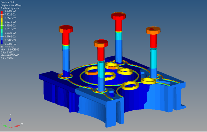
A contour plot of displacements is created, as shown in Figure 29. The cylinder head is hidden to view the displacement
plots for the head bolts.Figure 28. Displacement Contour for the Pressure Subcase after
Pretensioning
In Figure 29, the displacement plot after running the pressure
subcases can be seen. The maximum displacement is around 0.089 mm and it
occurs in the region near the pretensioned bolt heads.
Select Gasket Thickness-direction Pressure in the
Contour panel and click
Apply.
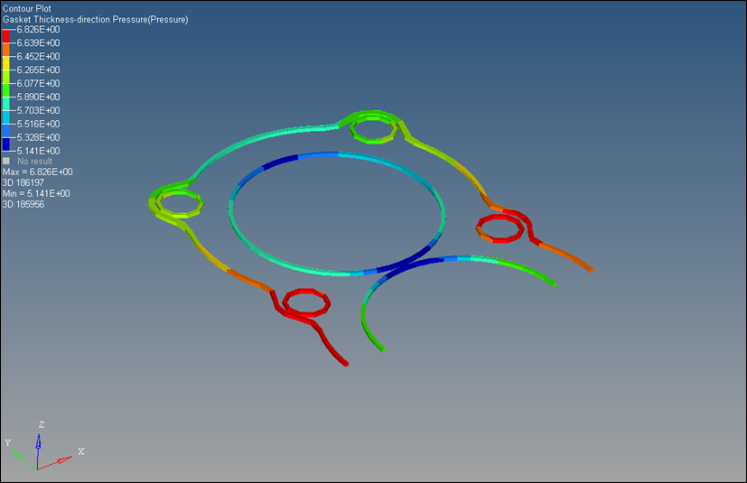
A contour plot of gasket pressure in the thickness direction is created, as
shown in Figure 30. The other components are hidden to be able to better
view the pressure variation on the gasket.Figure 29. Gasket pressure in the thickness direction for the Pressure
subcase
Checkpoint
The maximum pressure on the Gasket in the thickness direction is equal to
0.21 MPa.

 to view
the predefined contact surface PT_Surf on the third bolt.
Tip: If the predefined surface is not visible, then switch on (show) the PT_Surf entry in the Model Browser by clicking on the
to view
the predefined contact surface PT_Surf on the third bolt.
Tip: If the predefined surface is not visible, then switch on (show) the PT_Surf entry in the Model Browser by clicking on the icon next to it.
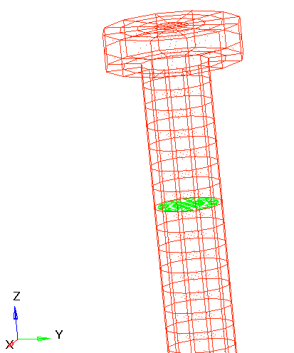
 next to the BLOCK and CYLINDER_HEAD components in the
Model Browser to show the hidden components.
next to the BLOCK and CYLINDER_HEAD components in the
Model Browser to show the hidden components.
 to add it to the selected nonlinear parameter:
section.
to add it to the selected nonlinear parameter:
section.

 .
.