This kind of analysis provides an estimate of peak structural response to a structure
subject to dynamic excitation. The analysis uses response spectra for prescribed
dynamic loading and results of normal modes analysis to calculate this estimate.
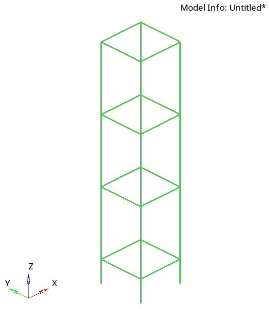
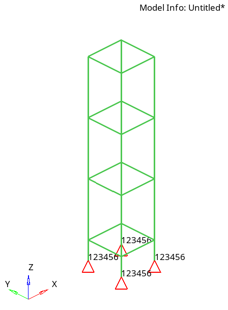
In the model used shown in Figure 1, a building structure is modeled using CBEAM
elements having solid circular x-section (that is type 'ROD'). The base of the
building structure will be constrained for all degrees of freedom and the structure
will be excited in the global Z direction.Figure 1. Building Structure HyperMesh
Model
Launch HyperMesh and Set the OptiStruct User Profile
Launch HyperMesh.
The User Profile dialog opens.
Select OptiStruct and click
OK.
This loads the user profile. It includes the appropriate template, macro
menu, and import reader, paring down the functionality of HyperMesh to what is relevant for generating models for
OptiStruct.
Open the Model
Click File > Open > Model.
Select the building_ResponseSpectrumAnalysis.hm file you saved to
your working directory.
Click Open.
The building_ResponseSpectrumAnalysis.hm database is loaded
into the current HyperMesh session, replacing any
existing data.
Set Up the Model
Create EIGRL Load Step Input
Define the EIGRL card to calculate the normal modes of the model.
In the Model Browser, right-click and select Create > Load Step Inputs.
For Name, enter eigrl_card.
For Config type, select Real Eigen Value
Extraction.
For Type, select EIGRL from the drop-down menu.
Click ND and enter a value of
10.
Create Constraints
In the Model Browser, right-click and select Create > Load Collector from the context menu.
A default load collector displays in the Entity Editor.
For Name, enter constraints.
Click Color and
select a color from the color palette.
For Card Image, select None from the drop-down
menu.
Go to the Analysis page.
Click constraints.
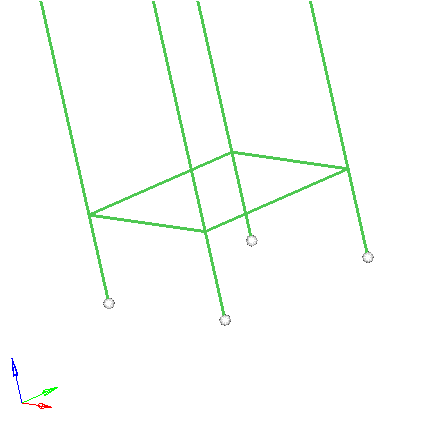
In the create subpanel, confirm the entity is set to nodes , click on nodes and
select the 4 nodes at the bottom of the model, as shown.
Figure 2. Selecting Nodes for Defining Constraints
Check all dofs (that is, dof1 to dof6) with the value 0.000, confirm load types
is set to SPC, and click create.
The constraints are created as shown in the figure below.Figure 3. Constraints Defined for the Model
Click return to exit the Constraints panel.
Define the Input Response Spectrum
Go to the Utility tab. If the Utility menu is not displayed, select View > Browsers > HyperMesh > Utility.
At the bottom of the Utility menu, click the
FEA panel.
Under Tools, click TABLE Create.
Select Import Table under Options and
TABLED1 under Tables.
Click Next.
Under Options, select Create New Table.
For Name, enter tabled1_card.
Click Browse.
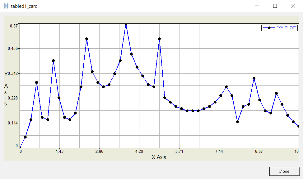
For Files of type: change to CSV (*.csv), select the file
sourceFileTABELD1.csv (which contains the 'x' and 'y'
values to define the input response spectrum, with frequency plotted on the
x-axis and acceleration on the y-axis) located in your working directory.
Click Open. If the Import TABLED1 GUI is minimized,
click on it on the taskbar.
In the Import TABLED1 GUI, click Apply.
A message is displayed indicating the creation of the
TABLED1 card.
Click OK for this message.
Click Exit on the Import TABLED1 GUI (if you do not see
the GUI, check the taskbar and click on the Import
TABLED1 GUI).
To see the plot corresponding to the TABLED1 card created
above, open the TABLE Create on the Utility menu on the
FEA panel.
Select the option Create/Edit Table.
For Tables select TABLED1.
Under Options, select Edit Existing Table.
Next to Select, select tabled1_card and click
Plot.
After reviewing the plot, click on Close in the
Plot window and Exit on
the Create/Edit TABLED1 GUI.
Figure 4. Plot of the TABLED1 Card
Define the DTI, SPECSEL Card
This card specifies the type of spectrum and damping values associated with the input
response spectrum defined using TABLED1 card in the previous
step.
Click the Model tab to bring up the Model Browser.
In the Model Browser, right-click and select Create > Load Collector from the context menu.
A default load collector displays in the Entity Editor.
For Name, enter dti_card.
For Card Image, select DTI.
For TYPE, select A, since the input response spectrum is
a plot of acceleration v/s frequency.
Click the Table icon next to the Data field. In the
pop-out window, select tabled1_card for
TID(1) and enter 0.02 for
DAMP(1).
The damping value is in the units of fraction of critical damping.
Define the RSPEC Load Collector
This card provides the specifications of the Response Spectrum Analysis.
In the Model Browser, right-click and select Create > Load Collector from the context menu.
A default load collector displays in the Entity Editor.
For Name, enter rspec_card.
For Card Image, select RSPEC.
For directional combination method, DCOMB, select
ALG.
For modal combination method, MCOMB, select SRSS.
Click CLOSE and enter a value of
1.000 in the input box.
For RSPEC_NUM_DTISPEC, enter 1.
Click next to Data. In the pop-out window, select
dti_card for the DTISPEC field, and for SCALE, enter
the value 9800.0.
Since the direction of excitation for the structure is the Global Z direction,
enter 0.0 for X(0), 0.0 for X(1),
and 1.0 for X(2), respectively.
Click Close to exit the window.
Define the Modal Damping for the Structure
In the Model Browser, right-click and select Create > Curve.
A new Curve editor window opens.
For Name, enter tabdmp1_card.
Enter the values 0.0, 0.02,
50.0 and 0.02 for x(1), y(1),
x(2) and y(2), respectively in the window.
Click Close to exit the window.
In the Model Browser, under Curves, select
tabdmp1_card.
For Card Image, select TABDMP1.
For TYPE, select CRIT.
Define the PARAM Cards
On the Analysis page, click control cards panel, click
next twice, and then click
PARAM panel.
Scroll down the list of available params, check the box next to
COUPMASS, and for the value, select
YES, so the coupled mass matrix approach is used for
eigenvalue analysis.
Scroll down the list of available params, check the box next to
EFFMASS, and for the value, select
YES, so the modal participation factors and effective
mass are computed and output to the .out file.
Click return to exit the panel.
Define the Output Request
Displacements are output by default.
To output stress from the Analysis page, enter the control
cards panel.
Click next to the page which has the
GLOBAL_OUTPUT_REQUEST panel.
Click GLOBAL_OUTPUT_REQUEST, scroll down the list to
STRESS and check it.
For OPTION(1), select ALL.
Click return twice to exit the control cards
panel.
Define the Response Spectrum Analysis Load Step
In the Model Browser, right-click and select Create > Load Step from the context menu.
For Name, enter response_spec.
Click Analysis type and select Response
spectrum from the drop-down menu.
For SPC, click Unspecified > Loadcol.
In the Select Loadcol dialog, select
constraints from the list of load collectors and
click OK.
For RSPEC, click Unspecified > Loadcol.
In the Select Loadcol dialog, select
rspec_card from the list of load collectors and click
OK.
For METHOD(STRUCT), click Unspecified > Load step inputs.
In the Select Load step inputs dialog,
select eigrl_card from the list of
load step inputs and click OK.
For SDAMPING(STRUCT), click Unspecified > Curves.
In the Select Curves dialog, select
tabdmp1_card from the list of
curves and click OK.
Click return to exit the Loadsteps panel.
From the Analysis page, enter the
OptiStruct panel.
Click Save as following the input file:
field. A Save file browser window opens.
Select the directory where you would like to write the file and enter the name for the file in the File name: field.
Note: Save the file in a folder different from the folders under Altair HyperWorks installation
folder.
Click Save.
Note: The name and location of the file displays
in the input file: field.
Set the export options: toggle to
all.
Set the run options: toggle to
Analysis.
Set the memory options: toggle to memory
default.
Click
OptiStruct. This launches the
OptiStruct job.
If the job completed successfully, new results files can be
seen in the directory where the OptiStruct model file was
written. The .out file is a good place
to look for error messages that will help to debug the input
deck if any errors are present and this can be done by
clicking on the view .out button in
the OptiStruct panel.
Submit the Job
From the Analysis page, click the OptiStruct
panel.
Figure 5. Accessing the OptiStruct Panel
Click save as.
In the Save As dialog, specify location to write the
OptiStruct model file and enter
building_ResponseSpectrumAnalysis for filename.
For OptiStruct input decks,
.fem is the recommended extension.
Click Save.
The input file field displays the filename and location specified in the
Save As dialog.
Set the export options toggle to all.
Set the run options toggle to analysis.
Set the memory options toggle to memory default.
Click OptiStruct to launch
the OptiStruct job.
If the job is successful, new results files
should be in the directory where the building_ResponseSpectrumAnalysis.fem was written. The building_ResponseSpectrumAnalysis.out file is a good place to look for error messages that could help
debug the input deck if any errors are present.
View the Results
From the OptiStruct panel, click HyperView.
HyperView is launched and the results are
loaded. A message window appears to inform of the successful model and result
files loading into HyperView.
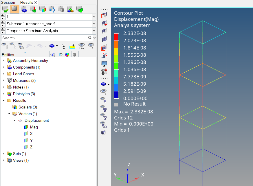
In the HyperViewResults Browser, expand the Results folder, then expand the
Vector folder and contour displacement results by selecting
Mag under Displacement.
Figure 6. Displacement Contour
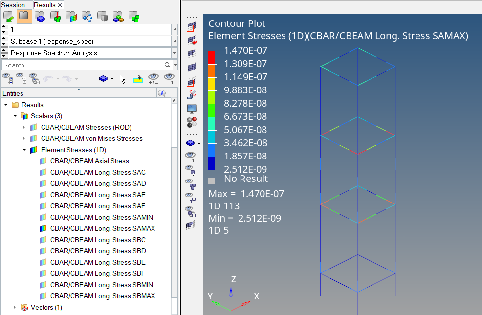
To contour stresses, expand the Scalar folder under Results, expand Element
Stresses (1D) and contour the stress you want to see.
Shown below is the contour of CBAR/CBEAM Long.Stress SAMAX.Figure 7. Stress Contour

 , click on nodes and
select the 4 nodes at the bottom of the model, as shown.
, click on nodes and
select the 4 nodes at the bottom of the model, as shown.
 next to the Data field. In the
pop-out window, select tabled1_card for
TID(1) and enter 0.02 for
DAMP(1).
The damping value is in the units of fraction of critical damping.
next to the Data field. In the
pop-out window, select tabled1_card for
TID(1) and enter 0.02 for
DAMP(1).
The damping value is in the units of fraction of critical damping.