
OS-T: 1372 Rotor Dynamics of a Hollow Cylindrical Rotor
In this tutorial you will perform Rotor Dynamics analysis on a hollow cylindrical rotor.
For rotating components, additional forces like the gyroscopic force and circular damping force exist and are critical in the study of their response. It is important to determine these effects of rotating components on the system as a whole. Here the complex eigenvalue analysis for 0, 10K, 30K, and 50K RPM are run.
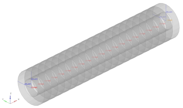
- 1D Line Mesh is created using beam elements for the Rotor
- Rotor is defined with Material MAT1
- Rotor is defined with Beam Property
- SPC condition is defined in the model
Figure 2. 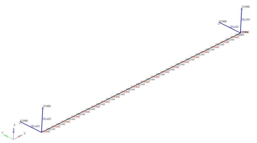
Launch HyperMesh and Set the OptiStruct User Profile
-
Launch HyperMesh.
The User Profile dialog opens.
-
Select OptiStruct and click
OK.
This loads the user profile. It includes the appropriate template, macro menu, and import reader, paring down the functionality of HyperMesh to what is relevant for generating models for OptiStruct.
Import the Model
-
Click .
An Import tab is added to your tab menu.
- For the File type, select OptiStruct.
-
Select the Files icon
 .
A Select OptiStruct file browser opens.
.
A Select OptiStruct file browser opens. - Select the rotor.fem file you saved to your working directory.
- Click Open.
- Click Import, then click Close to close the Import tab.
Set Up the Model
Create EIGRL and EIGC Cards
- In the Model Browser, right-click and select .
- In the Name field, enter EIGRL.
- For Config type, select Real Eigen Value Extraction.
- For Type, select EIGRL from the drop-down menu.
-
Click V2 and input 250.0.
250.0 is defined as the highest frequency bond.
- Create another load step input named EIGC.
- For Config type, select Complex Eigen Value Extraction.
- For Type, verify the default EIGC is selected.
-
Click NORM and select MAX.
MAX option is used to normalize the eigenvectors.
- For ND0 OPTIONS, select User Defined from the drop-down menu.
-
Click ND0 and input 55.
The desired number of roots to be extracted is 55.
Define Grids for the Rotor Line Model
- Right-click in the Model Browser and select .
- Click Name and enter ROTORG_SET.
- Click Card Image and select ROTORG from the drop-down menu.
- Click Entity IDs and click on nodes.
- Select nodes by collector and select CBEAM, and proceed.
- Check the box next to the RSPINR field since every rotor defined via ROTORG requires a corresponding RSPINR entry.
- Click the field next to GRIDA and then Node.
- In the selection panel, click Node and enter 10000 in the ID= field.
- Similarly, for GRIDB, enter 10001.
- Click on the field next to SPTID and enter 1.0.
Create RSPEED Load Collector
- In the Model Browser, right-click and select .
- Click Name and enter RSPEED.
- Click Card Image and select RSPEED from the drop-down menu.
- Click S1 and enter 0.0, which is first reference rotor speed.
- Click DS and enter 10000.0, which is increment in reference rotor speed.
- Click NDS and enter 5, which is the number of reference rotor speed increments.
Create RGYRO Load Step Inputs
- In the Model Browser, right-click and select .
- Click Name and enter RGYRO.
- Click Config type and select Rotordynamic Analysis Parameters from the drop-down menu.
- For Type, verify RGYRO is selected.
-
Click SYNCFLG and select ASYNC
from the drop-down menu.
Tip: This is set to run an Asynchronous Rotor dynamics analysis.
- Click REFROTR and click set.
- Select ROTORG_SET and click OK.
- Check the field next to SPEED_ID.
- Next to the SPEED field, click and select RSPEED from the pop-up window.
Define Load Step for Modal Complex Eigenvalue Analysis
- In the Model Browser, right-click and select .
- In the Name field, enter Rotor Dynamics.
- Click Analysis type and select Complex eigen (modal) from the drop-down menu.
- For SPC, select SPC from the list of load collectors.
- For CMETHOD, select EIGC from the list of load step inputs.
- For METHOD(STRUCT), select EIGRL from the list of load step inputs.
- Under SUBCASE OPTIONS, check the field next to RGYRO and then RGYRO_ID.
- Click on the field next to ID to select load step input RGYRO.
Submit the Job
-
From the Analysis page, click the OptiStruct
panel.
Figure 3. Accessing the OptiStruct Panel 
- Click save as.
-
In the Save As dialog, specify location to write the
OptiStruct model file and enter
rotor_async for filename.
For OptiStruct input decks, .fem is the recommended extension.
-
Click Save.
The input file field displays the filename and location specified in the Save As dialog.
- Set the export options toggle to all.
- Set the run options toggle to analysis.
- Set the memory options toggle to memory default.
- Click OptiStruct to launch the OptiStruct job.
Run the Model
- Click on the RGYRO card in the Model Browser.
- Click SYNCFLG and change from ASYNC to SYNC from the drop-down menu.
- From the Analysis page, enter the OptiStruct panel.
-
Click Save as following the input file:
field.
A Save As browser window opens.
- Select the directory where you would like to write the file and enter the name rotor_sync.fem in the File name: field.
-
Click Save.
Note: The name and location of the file displays in the input file: field.
- Set the export options: toggle to all.
- Set the run options: toggle to Analysis.
- Set the memory options: toggle to memory default.
- Click OptiStruct. This launches the OptiStruct job.
If the job completed successfully, new results files can be seen in the directory where the OptiStruct model file was written. The rotor_sync.out file is a good place to look for error messages that will help to debug the input deck if any errors are present.
View the Results
-
Read the rotor_async.out in HyperView.To get the Campbell Diagram and review the
critical frequencies at the intersection points, select Campbell Diagram Instructions.
Figure 4. 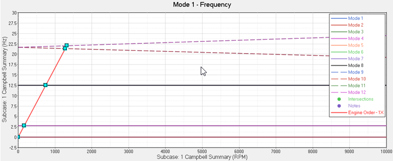
TableView in HyperView provides a summary for the critical frequencies.Figure 5. 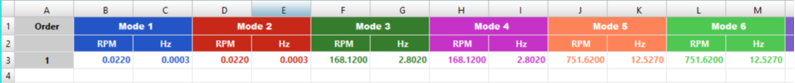
-
Load the rotor_sync.out
file in a text editor.
The Frequencies which you get from the Synchronous Rotor dynamic analysis give you the critical frequencies. The complex modes contain the imaginary part, which represents the cyclic frequency, and the real part which represents the damping of the mode. If the real part is negative, then the mode is said to be stable. If the real part is positive, then the mode is unstable.
Figure 6. Eigenvalues of the Complex Modes 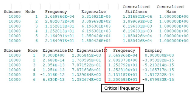
- Compare to verify the Critical Frequencies which you obtained from the intersection points and the frequencies you obtained in the rotor_sync.out file.
-
Load the rotor_async.h3d
file into HyperView to
review and verify below Cylindrical and Conical
mode shapes.
RPM Cylindrical Modes Forward Mode #3
Cylindrical Modes Backward Mode #4
Conical Modes Forward Mode #5
Conical Modes Backward Mode #6
10,000 2.802E+00 2.802E+00 1.248E+01 1.248E 30,000 2.802E+00 2.802E+00 1.201E+01 1.201E+01 50,000 2.802E+00 2.802E+00 1.058E+01 1.058E+1