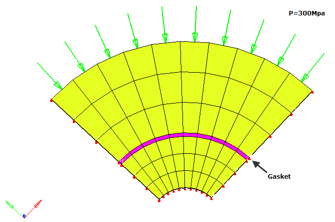
Figure 1 illustrates the structural model used for this tutorial: A 1mm
thick cylindrical gasket is sandwiched between two co-axial steel cylindrical tubes.
The outer cylinder is subjected to a pressure of 300 MPa on the outer surface as
shown. Using symmetry boundary conditions, only a quarter of the geometry has been
modeled. The gasket is connected to the inner and outer cylinders using contact.Figure 1. Model and Loading Description
Launch HyperMesh and Set the OptiStruct User Profile
Launch HyperMesh.
The User Profile dialog opens.
Select OptiStruct and click
OK.
This loads the user profile. It includes the appropriate template, macro
menu, and import reader, paring down the functionality of HyperMesh to what is relevant for generating models for
OptiStruct.
Open the Model
Click File > Open > Model.
Select the gasket_model.hm file you saved to
your working directory.
Click Open.
The gasket_model.hm database is loaded
into the current HyperMesh session, replacing any
existing data.
Set Up the Model
Create the Curves for Gasket Material
First, define the loading-unloading curves for the gasket material.
In the Model Browser, right-click and select Create > Curve.
A new Curve editor window opens.
For Name, enter load-curve.
In the X (closure) and Y (pressure) fields, enter the values shown in the table in step
6.
Close the curve editor window.
In the Curves select table, click Color and select a color from
the palette.
For Card Image, select TABLES1 from the drop-down menu.
For details on pressure-closure definitions of gaskets, refer to the Altair HyperWorks2024 online help.
For details on pressure-closure definitions of gaskets, refer to the Altair HyperWorks2024 online help.
X
Y
0.0
0.0
0.005
200.0
0.05
450.0
0.135
700.0
0.22
820.0
0.287
830.0
Now, unloading curves can be created.
Create the unloading curve named unload-curve1 with the
following X-Y data:
X
Y
0.08
0.0
0.12
140.0
0.135
700.0
Next, create the second unloading curve named
unload-curve2 with the
following X-Y data:
X
Y
0.17
0.0
0.2
250.0
0.22
820.0
Finally, create the third unloading curve named
unload-curve3 with the
following X-Y data:
X
Y
0.23
0.0
0.265
360.0
0.287
830.0
Create the Elasto-plastic Gasket Material
The membrane behavior of the gasket needs to be defined.
In the Model Browser, right-click and select Create > Material.
For Name, enter gask_membrane.
Click Color and
select a color from the color palette.
For Card Image, select MAT1 from the drop-down
menu.
For E, enter 2.0E+04 and for NU, enter
0.2.
Next, you will define the nonlinear properties for the gasket
material.
Create another material named gask_nonlin.
For Card Image, select MGASK.
Since this is an elasto-plastic gasket material, for gasket behavior leave
BEHAV field as 0.
For initial yield pressure, leave the YPRS field blank for the solver to
determine it automatically.
For tensile modulus EPL, enter 0.001.
For GPL to specify the shear modulus, enter 2000.
For MGASK_TABLU_NUM, enter 3 to specify the field for #
of unloading curves.
For TABLD, select load-curve.
Click next to the Data field and select the following:
TABLU(1)
unload-curve1
TABLU(2)
unload-curve2
TABLU(3)
unload-curve3
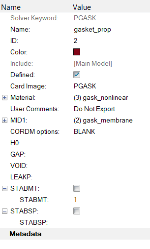
Create the Gasket Property
In the Model Browser, right-click and select Create > Property.
For Name, enter gasket_prop.
Click Color and
select a color from the color palette.
For Card Image, select PGASK from the drop-down menu and
click Yes to confirm.
For Material, click Unspecified > Material.
In the Select Material dialog, select
gask_nonlin from the list of materials and click
OK to complete the selection.
For MID1, select the gask_membrane material.
For STABMT field, select 1 to define some stabilization
stiffness.
Figure 2.
Next, assign this property to the gasket component. Click on the component
GASKET in the Model Browser.
For Property, select gasket_prop property.
Assign 8-Noded Gasket Elements
Click on the 3D page from the main menu.
Click the elem types panel and click 2D &
3D.
Click on elems, select by collector
type and select the GASKET
component.
Toggle hex8 =, and select the
CGASK8 element type.
Click update > return.
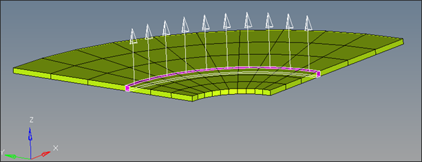
Review and Adjust the Normals of the Gasket Elements
Click on 2D page from the main menu.
Click on the composites panel.
For comps, select the GASKET component and click
display normals.
The normals of the gasket elements are not in the thickness direction, but in
the Z-direction, as shown below.Figure 3.
So, adjusting the normals needs to be in thickness
direction.
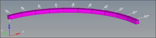
Display only the GASKET component.
Click on by nodes on bottom face and select the
GASKET component.
For choosing the face nodes, click on nodes and select
three nodes on a face of any gasket element in the thickness direction and click
adjust normals.
The normals are now adjusted to be in thickness direction of gasket, as
shown below.Figure 4.
Click return to go back to the main menu.
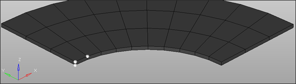
Define Contact between the Cylinders and Gasket
Now the contact surface for the bottom surface of the top cylinder needs to be
defined.
Hide the GASKET component and display only
the SOLID1 component.
In the Model Browser,
right-click and select Create > Set Segment.
For Name, enter
SOLID1_bottom.
Click Color and
select a color from the color palette.
For Card Image, select
SURF from the drop-down
menu.
Click on Elements and
on the yellow Elements
panel.
Under the modeling window, select
add solid faces from the
selection menu.
Click elems >>
displayed.
Click on face nodes,
select the three nodes on the bottom surface (that
is, the surface contacting the gasket, as shown
below) and click add.
Figure 5.
Click return.
Next, hide the SOLID1 component and display
only the SOLID2 component.
Create the set segment
SOLID2_top for the top
surface of the SOLID2 component contacting the
gasket.
Similarly, repeat the steps and create
GASKET_top and
GASKET_bottom segments for
the top and bottom surfaces of the GASKET
component, respectively.
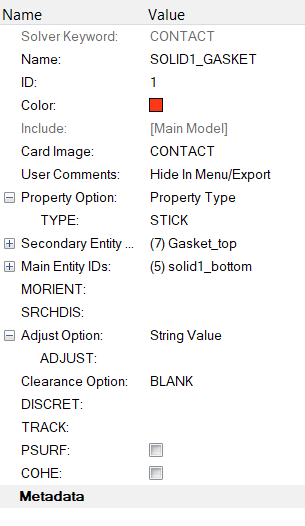
Now, an interface between the top
cylinder and gasket are created.
In the Model Browser,
right-click and select Create > Contact.
For Name, enter
SOLID1_GASKET.
Click Color and
select a color from the color palette.
For Card Image, select
CONTACT from the drop-down
menu.
For Main Entity IDs, select the
SOLID1_bottom
surface.
For Secondary Entity IDs, select the
GASKET_top surface.
For TYPE, select STICK
from the drop-down menu.
Figure 6.
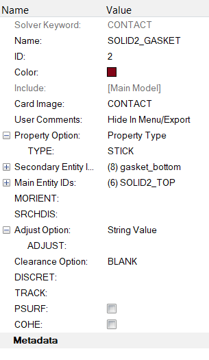
Next, an interface between the bottom cylinder
and gasket are created.
In the Model Browser,
right-click and select Create > Contact.
For Name, enter
SOLID2_GASKET.
Click Color and
select a color from the color palette.
For Card Image, select
CONTACT from the drop-down
menu.
For Main Entity IDs, select the
SOLID2_top surface.
For Secondary Entity IDs, select the
GASKET_bottom
surface.
For TYPE, select STICK
from the drop-down menu.
Click review to review
the interface.
Figure 7.
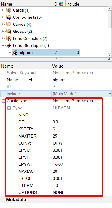
Define Nonlinear Implicit Parameters
In the Model Browser, right-click and select
Create > Load Step Inputs.
For details on the nonlinear implicit parameters, refer to the online
help.
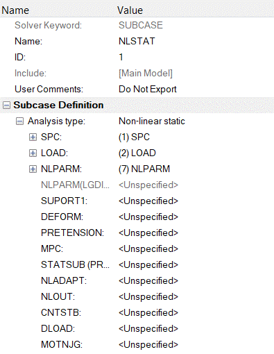
Create NLSTAT Load Step
In the Model Browser, right-click and select Create > Load Step.
For Name, enter NLSTAT.
Click Color and
select a color from the color palette.
Click Analysis type and select Nonlinear static from the
drop-down menu.
For SPC, select SPC from the list of load
collectors.
For LOAD, select LOAD from the list of load
collectors.
For NLPARM, select NLPARM from the list of load step
inputs.
Figure 9.
Define Output Control Parameters
From the Analysis page, select control cards.
Click on GLOBAL_OUTPUT_REQUEST.
Below CONTF, DISPLACEMENT, STRAIN and STRESS, set Option to
Yes.
Click return twice to go to the main menu.
Submit the Job
From the Analysis page, click the OptiStruct
panel.
Figure 10. Accessing the OptiStruct Panel
Click save as.
In the Save As dialog, specify location to write the
OptiStruct model file and enter
gasket_complete for filename.
For OptiStruct input decks,
.fem is the recommended extension.
Click Save.
The input file field displays the filename and location specified in the
Save As dialog.
Set the export options toggle to all.
Set the run options toggle to analysis.
Set the memory options toggle to memory default.
Click OptiStruct to launch
the OptiStruct job.
If the job is successful, new results files
should be in the directory where the gasket_complete.fem was written. The gasket_complete.out file is a good place to look for error messages that could help
debug the input deck if any errors are present.
View the Results
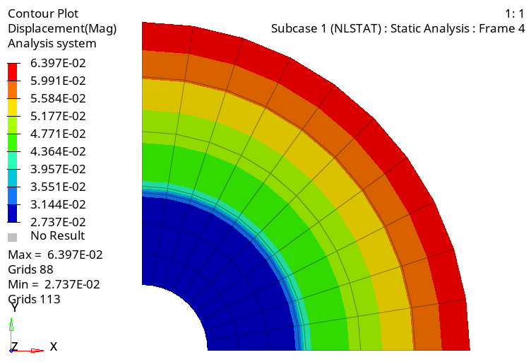
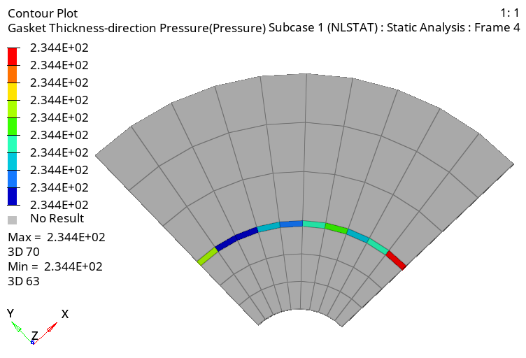
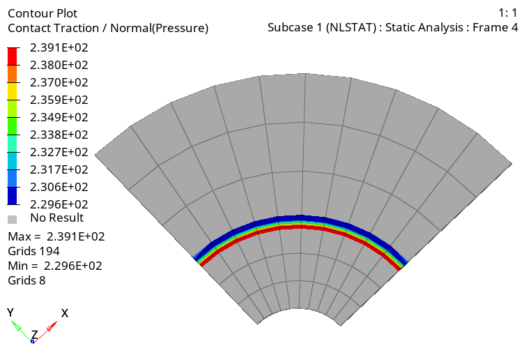
In HyperView, plot the displacement and contact pressure
contours at the end of the analysis.Figure 11. Contour of Displacements in Cylinders and Gasket Subject to Loading Figure 12. Contour of Gasket Thickness Direction Pressure Figure 13. Contour of Contact Pressure

 next to the Data field and select the following: