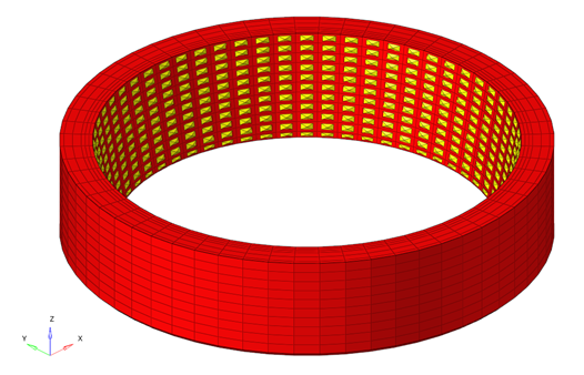
This tutorial demonstrates the heat transfer analysis on a set of piston rings (Figure 1).
The inner ring takes the heat flux (10.0W/m2) from the piston. The outer surface
of the ring that contacts the cylinder wall is maintained at a temperature of 0° C. The heat
transfer is modeled by using thermal contact definition between the two rings.
The thermal boundary condition, heat flux loading, and a linear steady-state heat
conduction subcase have already been defined in the initial base model. The focus of this
tutorial is on defining the thermal contacts between the rings.Figure 1. Piston Ring Arrangement
The following exercises are included in this tutorial:
Define contact surfaces between the rings
Define thermal contact at the interface
Solve the heat conduction analysis with OptiStruct solver
Post-process the results in HyperView
Launch HyperMesh and Set the OptiStruct User Profile
Launch HyperMesh.
The User Profile dialog opens.
Select OptiStruct and click
OK.
This loads the user profile. It includes the appropriate template, macro
menu, and import reader, paring down the functionality of HyperMesh to what is relevant for generating models for
OptiStruct.
Import the Model
Click File > Import > Solver Deck.
An Import tab is added to your tab menu.
For the File type, select OptiStruct.
Select the Files icon .
A Select OptiStruct file browser
opens.
Select the Rings.fem file you saved
to your working directory.
Click Open.
Click Import, then click Close to
close the Import tab.
Set Up the Model
Create Set Segments Between the Rings
In this step, the contact surfaces will be created, and the thermal contact will be
defined.
In the Model Browser, right-click and select Create > Set Segment.
For Name, enter RING1 inner surface.
Click the Elements Selection and click add solid faces
option to select faces in the inner surface of RING1, as shown in Figure 3.
Figure 2. Selection of solid faces from the toolbar Figure 3. Contact surface on the inner surface of Ring 1
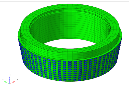
Similarly, repeat the same process to define contact faces on the outer surface
of RING2.
For Name, enter RING2 outer surface.
Figure 4. Contact surface on the outer surface of Ring 2
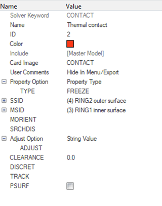
Create Thermal Contacts Between the Rings
In this step, the thermal contacts will be defined between the rings.
In the Model Browser, right-click and select Create > Groups.
For Name, enter Thermal contact.
In the Property Option, click Property Type and select
FREEZE from the drop-down menu.
For SSID, select RING2 outer surface.
For MSID, select RING1 inner surface.
For CLEARANCE field, enter 0.0.
This will help close the contact; thereby, ensuring the heat transfer
across the interface.
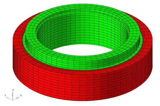
As described at the beginning of this tutorial, the
heat transfer boundary condition (Temp RING2 outer), heat flux input (Heat
flux) are already in the model. An OptiStruct
steady-state heat conduction loadstep, referring to the boundary condition
and flux, has been defined, as well. The heat transfer results are requested
in loadsteps panel. Refer to tutorial OS-T: 1080 for the
details on how to define heat transfer boundary condition, heat flux, and
the output request.
Note: Without the thermal contact, the heat transfer
would not occur at the interface of the rings. In this case, the outer
ring would remain at zero temperature and the inner ring would take all
the heat.
Figure 5. Contact definition between the ring
Submit the Job
From the Analysis page, click the OptiStruct
panel.
Figure 6. Accessing the OptiStruct Panel
Click save as.
In the Save As dialog, specify location to write the
OptiStruct model file and enter
Rings_complete for filename.
For OptiStruct input decks,
.fem is the recommended extension.
Click Save.
The input file field displays the filename and location specified in the
Save As dialog.
Set the export options toggle to all.
Set the run options toggle to analysis.
Set the memory options toggle to memory default.
Click OptiStruct to launch
the OptiStruct job.
If the job is successful, new results files
should be in the directory where the Rings_complete.fem was written. The Rings_complete.out file is a good place to look for error messages that could help
debug the input deck if any errors are present.
Post-process the Results
Temperature and flux contour results for the steady-state heat conduction analysis are
computed by OptiStruct. HyperView will be used to post-process the results.
From the OptiStruct panel, click HyperView.
HyperView is launched and the results are
loaded. A message window appears to inform of the successful model and result
files loading into HyperView.
Click Close to close the message window, if one
appears.
On the Results toolbar, click to open the
Contour panel.
Select Subcase 1 - heat transfer as the current load
case in the Load Case and Simulation Selection
window.
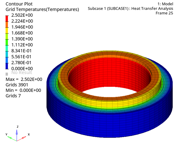
Select the first pull-down menu below Result type and select Grid
Temperatures(s).
Click Apply.
A temperature contour plot is now available.
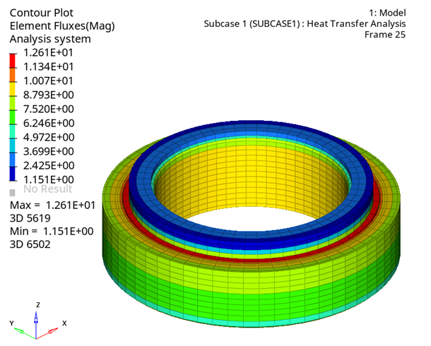
Select the first pull-down menu below Result type and select Element
Fluxes(V).
Click Apply.
Both temperature and flux results are shown below.Figure 7. Grid Temperature Plot Figure 8. Element Flux Plot

 .
A Select OptiStruct file browser opens.
.
A Select OptiStruct file browser opens.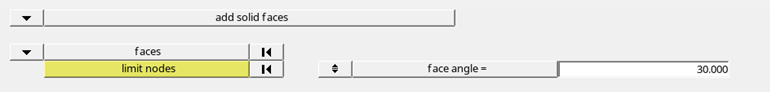

 to open the
Contour panel.
to open the
Contour panel.