The flat plate is subjected to a frequency-varying unit load
excitation using the direct method. Post-processing is done
in HyperView and HyperGraph to visualize
deformations, mode shape response, and frequency-phase
output characteristics.
Launch HyperMesh and Set the OptiStruct User Profile
Launch HyperMesh.
The User Profile dialog opens.
Select OptiStruct and click
OK.
This loads the user profile. It includes the appropriate template, macro
menu, and import reader, paring down the functionality of HyperMesh to what is relevant for generating models for
OptiStruct.
Import the Model
Click File > Import > Solver Deck.
An Import tab is added to your tab menu.
For the File type, select OptiStruct.
Select the Files icon .
A Select OptiStruct file browser
opens.
Select the direct_response_flat_plate_input.fem file you saved
to your working directory.
Click Open.
Click Import, then click Close to
close the Import tab.
Set Up the Model
Apply Loads and Boundary Conditions
In the following steps, the model is constrained at one edge. A unit vertical load is
applied acting upwards in the positive z-direction at a point on a free edge corner of
the plate.
Click the Model
tab.
In the Model Browser,
right-click and select Create > Load Collector.
For Name, enter
spcs.
Click Color and select a
color from the color palette.
Set the Card Image to
None.
A new load collector, spcs is
created.
In the Model Browser,
right-click and select Create > Load Collector.
For Name, enter
unit-load.
Click Color and select a
different color from the color palette.
A new load collector, unit-load is
created.
Create Constraints
In the Model Browser, expand Load
Collector, right-click spcs > Make Current.
Figure 1.
Click the Display Numbers icon .
Click nodes > displayed.
Select on (green button).
All of the node numbers on the flat plate should now be
displayed.
Click return to go back to the main menu.
Click BCs > Create > Constraints to open the Constraints menu.
Click the entity selection switch and select nodes from
the pop-up menu.
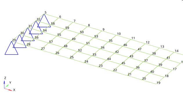
Click nodes and select nodes 5, 29, 30, 31 and 32 (Figure 2).
Figure 2. Nodes to Select for Applying Single Point Constraints
Constrain dof1, dof2,
dof3, dof4 and
dof5 (you only need to uncheck dof6).
DOFs with a check will be constrained while DOFs without a check will be
free.
DOFs 1, 2, and 3 are x, y, and z translation degrees of freedom.
DOFs 4, 5, and 6 are x, y, and z rotational degrees of freedom.
Click create.
The selected nodes will be free to rotate about the z-axis since dof6
was not checked.
Click return to go back to the main menu.
Create a Unit Load at a Point on the Flat Plate
In the Model Browser, right-click on the load collector
unit-load and select Make
Current.
From the Analysis page, click load types.
Select constraint = and select
DAREA from the extended entity selection menu.
Click return to exit the Load Types panel.
Click BCs > Create > Constraints to open the Constraints menu.
Select node number 19 on the plate by clicking on it (Figure 3).
Figure 3. Node Selected for Creating Unit Vertical Load
Uncheck all the dof's except dof3 and click the = to the
right of dof3 and enter a value of 20.
Click load types= and verify that DAREA is selected from
the extended entity selection menu.
Click create, and then click
return.
The unit load is applied to the selected node.
Create a Frequency Range Table
In the Model Browser, right-click and
select Create > Curve.
A new window opens.
For Name, enter tabled1.
In the table, enter x(1) = 0.0, y(1) =
1.0, x(2) = 1000.0, y(2) =
1.0.
Close the Curve Editor window.
From Curves, select tabled1.
For Type, select TABLED1
from the drop-down menu.
This provides a frequency range of 0.0 to 1000.0 with a constant 1.0 over
this range.
Create a Frequency Dependent Dynamic Load
In the Model Browser, right-click and select Create > Load Step Inputs.
For Name, enter rload2.
For Config type, select Dynamic Load – Frequency
Dependent from the drop-down list.
For Type, and select RLOAD2 from the
drop-down list.
For Excited, click Unspecified > Loadcol.
In the Select Loadcol dialog, select
unit-load from the list of load collectors and click
OK to complete the selection.
For TB, select the tabled1 curve.
The type of excitation can be an applied load (force or moment), an enforced
displacement, velocity or acceleration. The field Type in the RLOAD2 load step input defines the type of load. The
type is set to applied load by default.
Create a Set of Frequencies
In the Model Browser, right-click and
select Create > Load Collector.
For Name, enter freq1.
Click Color and
select a color from the color palette.
For Card Image, select FREQi from the
drop-down menu.
Check the FREQ1 option and enter
1 in the NUMBER_OF_FREQ1
field.
Update the following fields in the pop-out window.
For F1, enter 20.0.
For DF, enter 20.0.
For NDF, enter 49.
Click Close.
This provides a set of
frequencies beginning with 20.0, incremented by 20.0
and 49 frequencies increments.
Create a Load Step
In the Model Browser, right-click and
select Create > Load Step.
A default load step template is now displayed in the
Entity Editor below the
Model Browser.
For Name, enter subcase1.
For Analysis type, select Freq.resp (direct) from the drop-down
menu.
For SPC, select Unspecified > Loadcol.
From the Select Loadcol dialog, select
SPCS.
For DLOAD, select rload2 from the Select Load
Step Inputs pop-out window.
For FREQ, click Unspecified > Loadcol
From the Select Loadcol dialog, select
freq1.
An OptiStruct subcase has been
created which references the constraints in the load
collector spc and the unit load in the load
collector step input rload2 with a set of
frequencies defined in load collector freq1
Create a Set of Nodes
In the Model Browser, right-click and select Create > Set.
For Name, enter SETA.
For Card Image, select None.
Leave the Set Type switch set to non-ordered type.
For Entity IDs, select Nodes from the selection
switch.
Click Nodes and select nodes with IDs 15, 17 and 19.
Click proceed.
Create a Set of Outputs and Mass Factors
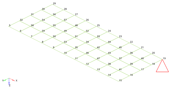
Click Setup > Create > Control Cards to open the Control Cards panel.
Select GLOBAL_OUTPUT_REQUEST and check
the box next to DISPLACEMENT.
Under FORM(1), select PHASE from the
pop-up menu.
Under OPTION(1), select SID from the
pop-up menu.
A new field appears in yellow.
Double-click the SID(1) box and select
SETA.
A value of 1 now appears below the SID field box. This
sets the output for only the nodes in set 1. Figure 4.
Click return to exit the
GLOBAL_OUTPUT_REQUESTS menu.
From the Control Cards panel, select
FORMAT.
A new window appears in the work area
screen.
Click number_of_formats = and input a
value of 2.
On the extended menu in the work area, click on the first
FORMAT_V1 field box and
select OPTI from the pop-up
menu.
Using OPTI generates OptiStructASCII result files like
.disp,
.strs, etc. as the output once
the run is complete. These files are used during
post-processing.
Make sure the second field box is set to H3D.
Click return to exit the Format menu and
return to the Control Cards menu.
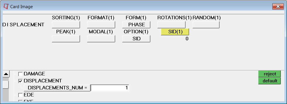
Click next and select the
PARAM subpanel.
Scroll down the list using the arrow in the left corner and
check the box next to COUPMASS.
A new PARAM card appears in the work
area screen.
Click NO below COUPM_V1 and select
YES from the pop-up menu
selection.
Selecting YES uses the coupled mass matrix approach for
eigenvalue analysis.
Scroll down the list using the arrow in the left corner and
check the box next to G.
A new PARAM card appears in the work
area screen.
Click below G_V1 and input a value of
0.06 into the field
box.
This value specifies a uniform structural damping coefficient
and is obtained by multiplying the critical damping [] ratio
by 2.0.
Scroll down using the arrow in the left corner and check the box next to WTMASS.
A new window appears in the work area
screen.
Click below WTM_V1 and input a value of
0.00259 into the field
box.
Three PARAM statements now appear in
the pop-up menu on the work screen. This factor is used to
input all mass entries in weight units. Using this
PARAM multiplies all terms in the
mass matrix by this factor.Figure 5.
Click return to exit the PARAM
menu.
Select the OUTPUT subpanel.
Verify that KEYWORD is set to
HGFREQ.
Using HGFREQ results in a frequency output presentation for
HyperGraph.
Click on the box beneath FREQ and select
ALL from the pop-up selection
to choose all outputs results for all frequencies.
Leave number_of_outputs set equal to 1.
Click return to exit OUTPUT.
Click return to exit the Control Cards
panel.
Submit the Job
From the Analysis page, click the OptiStruct
panel.
Figure 6. Accessing the OptiStruct Panel
Click save as.
In the Save As dialog, specify location to write the
OptiStruct model file and enter
flat_plate_direct_response for filename.
For OptiStruct input decks,
.fem is the recommended extension.
Click Save.
The input file field displays the filename and location specified in the
Save As dialog.
Set the export options toggle to all.
Set the run options toggle to analysis.
Set the memory options toggle to memory default.
Click OptiStruct to launch
the OptiStruct job.
If the job is successful, new results files
should be in the directory where the flat_plate_direct_response.fem was written. The flat_plate_direct_response.out file is a good place to look for error messages that could help
debug the input deck if any errors are present.
The default files written to the directory are:
flat_plate_direct_response.html
HTML report of the analysis, providing a
summary of the problem formulation and the analysis results.
flat_plate_direct_response.out
OptiStruct output file containing specific
information on the file setup, the setup of your optimization problem,
estimates for the amount of RAM and disk space required for the run,
information for each of the optimization iterations, and compute time
information. Review this file for warnings and errors.
flat_plate_direct_response.h3d
HyperView binary results file.
flat_plate_direct_response.res
HyperMesh binary results file.
flat_plate_direct_response.stat
Summary, providing CPU information for each step during analysis
process.
View the Results
This step describes how to view displacement results (.mvw file) in
HyperGraph and also explains the displacement output
(.disp file) from this run.
The HyperView results (.h3d file) contains
only the displacement results for the three nodes specified in the node set
output.
From the OptiStruct panel, click HyperView.
HyperView is launched and the results are
loaded. A message window appears to inform of the successful model and result
files loading into HyperView.
Click Close to close the message window, if one
appears.
In the HyperView window, click File > Open > Session.
The Open Session File window is
displayed.
Select the directory where the job was run and select the file flat_plate_direct_response_freq.mvw.
Click Open.
A warning appears asking whether to discard the existing
contents.
Click Yes.
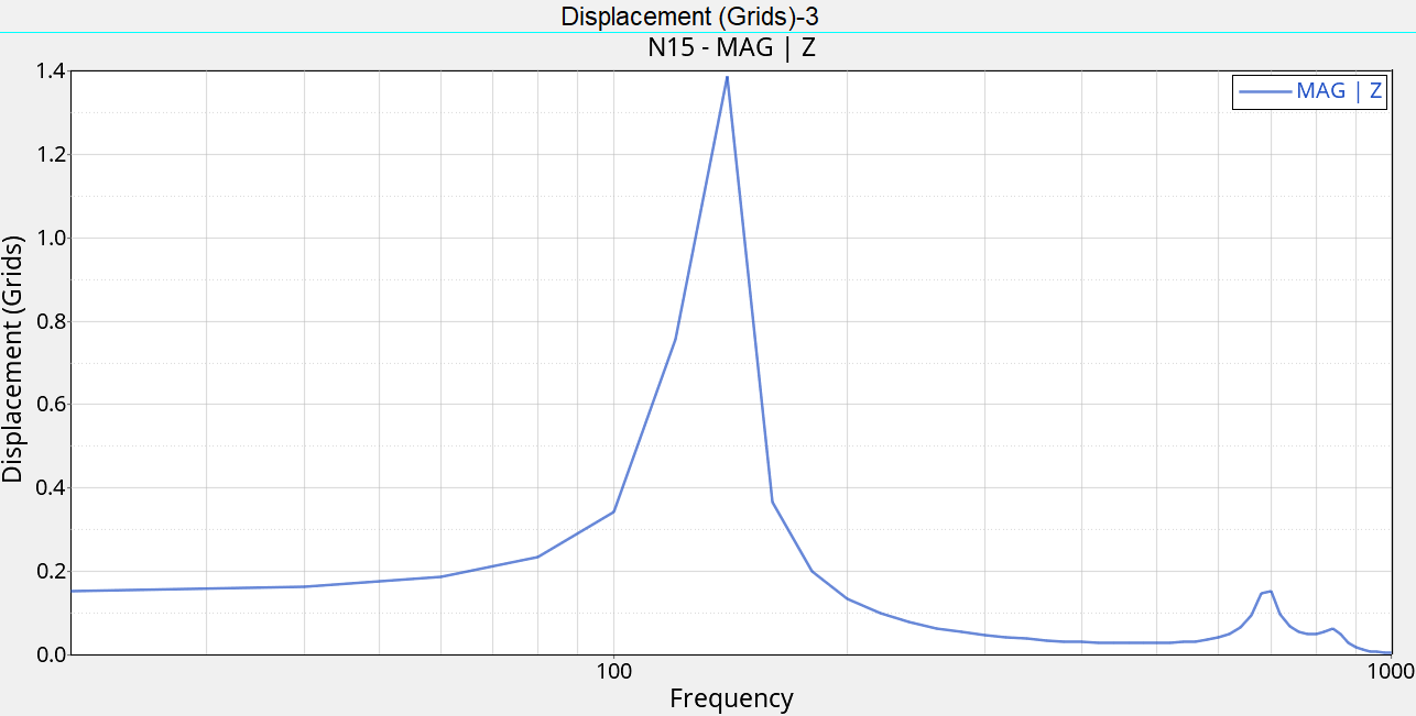
Two graphs per page and a total of three pages are displayed. The graph title
shows Subcase 1 Displacement of grid 15 on page 1.
There are two sets of
results on this page. The top graph shows Phase Angle verses Frequency
(log). The bottom graph shows Magnitude versus Frequency (log) (see Figure 7) for Displacement of grid 15.
Figure 7. Frequency Response of Node 15
Click the Next Page icon .
This displayed page 2, which shows Subcase 1 (subcase1) - Displacement of grid
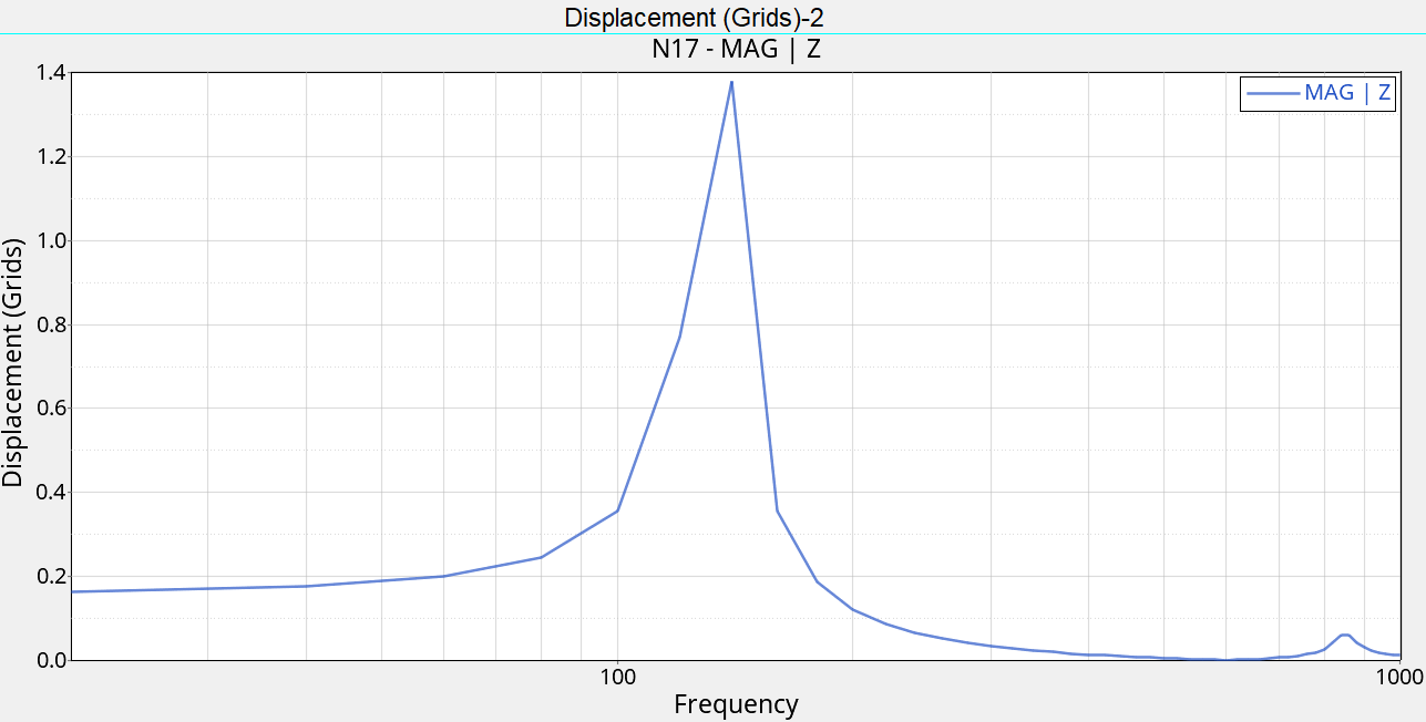
17 (Figure 8).Figure 8. Frequency Response of Node 17
Select the Next Page icon again to display page 3 containing Subcase 1 (subcase1)
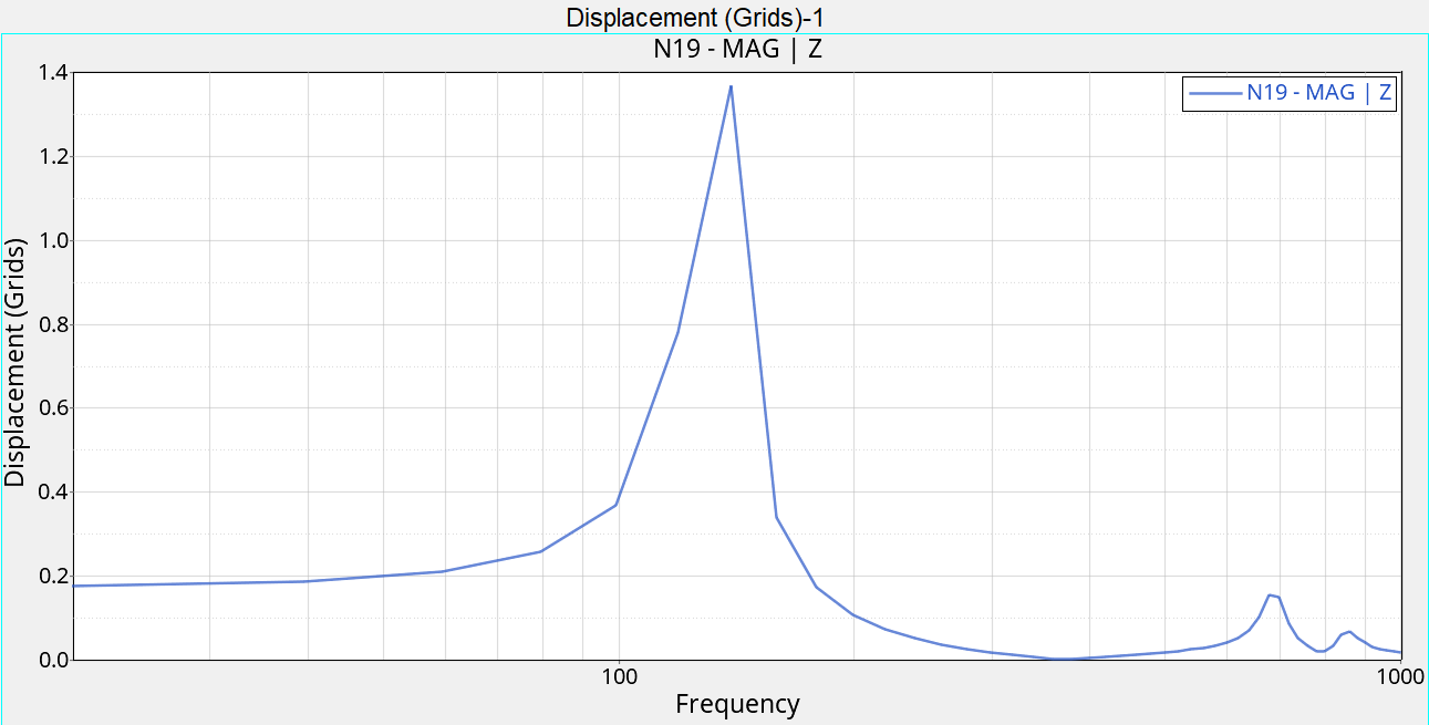
- Displacement of grid 19 (Figure 9).
Figure 9. Frequency Response of Node 19 This concludes the HyperGraph results
processing.
Open the displacement file (.disp) using a text editor.
The first field on the second line shows the iteration number, the second field shows the
number of data points, and the third field shows the iteration frequency.
Line
3, first field shows node number, then x, y, and z displacement magnitudes
and x, y and z rotation magnitudes.
Line 4, first field shows node
number, then x, y, and z displacement phase angles and x, y and z rotation
angles.

 .
A Select OptiStruct file browser opens.
.
A Select OptiStruct file browser opens.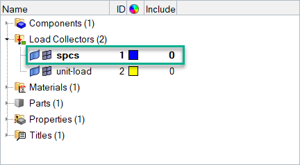
 .
.

 .
This displayed page 2, which shows Subcase 1 (subcase1) - Displacement of grid 17 (Figure 8).
.
This displayed page 2, which shows Subcase 1 (subcase1) - Displacement of grid 17 (Figure 8).