Introduction to MotionView - Part 2
Tutorial Level: Beginner This tutorial will teach you how to set up gravity, define bushings, and apply motion.
- Joints and Bushings
- Gravity
- Motion
- Redundant Constraint Removal
- Outputs
- Solve and Post-Process
Review the Solver Log File
-
Launch MotionView and open the
MV_intro1.mdl file that was saved in the previous
tutorial using the Open Model
 in the
Home group.
in the
Home group.
Or
Open the model by selecting .
Attention: In case you do not have the model and results of the previous tutorial, use the above link to download and execute a run to generate results. -
From the Ribbon bar, select Analyze and click on the
Run History satellite next to the Run icon from the
Solution group.
Figure 1. Run History Satellite Icon 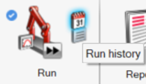
Note: The ‘Run History’ maintains the history of all runs per model. Model and results for the previous runs can be accessed through this tool.Expand the entry for the current model, right-click on the Run name MV_intro1_Run and click View Log.Figure 2. View Solver Log 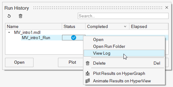
The solver log gets loaded in the text editor. Observe that there are two redundant constraints identified in the model.Figure 3. Solver Log Showing Two Redundant Constraints 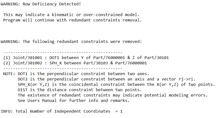
Each joint imposes a set of constraints or removes one or more degrees of freedom of the bodies based on their type. More details on the number of degrees of freedom removed by each joint type is available in the Joints topic. The current configuration of joints combined are such that there are more constraints than the total number of degrees of freedom in the model. MotionSolve is designed to detect redundant constraints and automatically remove them so that a unique solution can be found, and the simulation can proceed. However, such a simulation may:- Provide undesired or unexpected results.
- Mechanism lockups or simulation failures.
The recommended best practice is for you to review the model and remove the redundant constraints on your own. In the next steps, we will try to change the joint configurations to ensure that no redundant constraints are present.
- Close the Run History dialog.
-
Save the model using .
- Using the Save As Model dialog that appears, browse to your working directory and name the file MV_intro2.mdl.
- Click Save.
Redundant Constraint Removal
-
Select the joint Joint 1 from the Model Browser. In the Entity Editor,
change the following properties:
-
Label to
Crank-Conrod -
Varname to
j_crank_conrod
Note: If the Entity Editor is not visible by default, then turn it ON by performing a right-click on the joint from the Model Browser and selecting the Show Properties option from the context menu or use the Menu Bar, .Similarly, select the following joints one by one and rename their label and varname as per the following table:Current Label Current Varname Rename Label To Rename Varname To Joint 0 j_0 Crank j_crank Joint 2 j_2 Piston Pin j_pistonpin Joint 3 j_3 Piston-Cylinder j_piston_cyl Note: Varname is short for variable name, which is a unique identifier for an entity. Variable names can be used to relate the property of one entity to that of another entity.Similarly, select the Points one by one and rename them as per the following table:Current Label Current Varname Rename Label To Rename Varname To Point 0 p_0 Crank Center p_crank_cent Point 1 p_1 Crank-Conrod p_crank_conrod Point 2 p_2 Piston Pin p_pistonpin Point 3 p_3 Piston Pin Axis p_pistonpin_axis Point 4 p_4 Piston Center p_piston_cent -
Label to
-
Change the joint Piston Pin using the Entity Editor.
- Select the joint in the Model Browser.
- Change the Type to Universal.
- Under Orientation, change Alignment Type 1 to Shaft.
- Change Method 1 to Point.
- Activate Point 1 collector (below Method 1) and pick the Crank-Conrod point from the modeling window.
Figure 4. Changing Piston Pin to Universal Joint 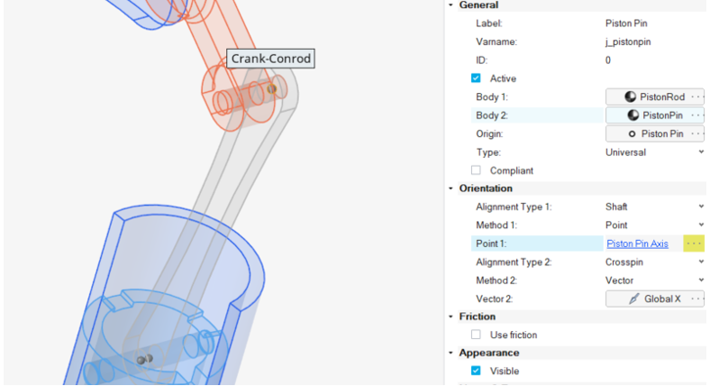
The Entity Editor after the change should be as shown in the below figure:Figure 5. Entity Editor of Piston Pin After Changes 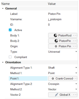
-
Change the joint type of Crank-Conrod. Through the
Entity Editor:
- Select the joint in the Model Browser.
- Change the Type to Cylindrical.
-
Run the model.
-
Click on the Analysis settings satellite icon
 near the Run ribbon icon.
-
Once the run is complete, review the log by selecting the Run name in
the Run Status dialog and clicking View
Log.
Figure 6. Accessing Log from the Run Status Dialog 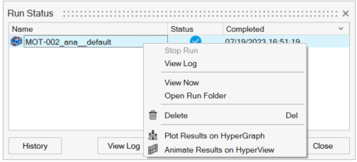
Note: The model behavior, as seen from the run animation, remains the same as before. Additionally, the Solver Log should not report any redundant constraint anymore. The previously reported redundant constraints have been effectively resolved by removing one constraint each from Crank-Crankrod joint and Piston Pin joint.Even though the chosen joint configuration has removed the redundant constraints, it may not represent the kind of joint interaction the parts have.
Other ways to resolve the redundant constraints situation are:- Change joint to Compliant (converts the joint into a force element called Bushing with stiffness and damping properties).
- Represent one of the bodies as a Flexible body.
Creation and usage of a flexible body will be covered in another tutorial. In the next step, Bushings and Compliant Joints will be explored.
-
Click on the Analysis settings satellite icon
Replace Joints with Bushings
-
Deactivate the joint Piston Pin.
- Select the joint from the Model Browser.
- Right-click and click .
Note: An entity can be deactivated by clearing the Active check box in the Entity Editor. -
Add a Bushing.
-
From the Model ribbon, click on the
Bushings icon
 under the Entities
group. Or use the search at the top right of the MotionView window to activate the bushing
creation context.
under the Entities
group. Or use the search at the top right of the MotionView window to activate the bushing
creation context.
Figure 7. Using Search to Find Functionalities 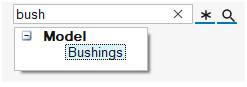
-
In the microdialog, click on the OrientMarker
tool
 .
.
- The Z axis is active for orientation. Change to 1-Axis method.
- Select the Point method
 in the microdialog.
 - Select the existing point Piston Pin
Axis.
Figure 8. Orienting Bushing Axis Using Existing Point 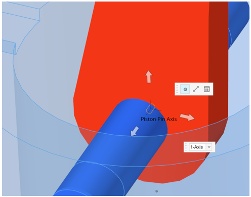
- Right-click in an empty space and click
Exit
 .
.
-
Click Cancel on the guide bar and click Exit
.
-
From the Model ribbon, click on the
Bushings icon
-
Modify bushing properties using the Entity Editor.
-
Change the Rot Stifness value (ktx and kty) to
1e8. Set Value(ktz) to0.0 N-mm/rad.Figure 9. Stiffness Properties of Bushing 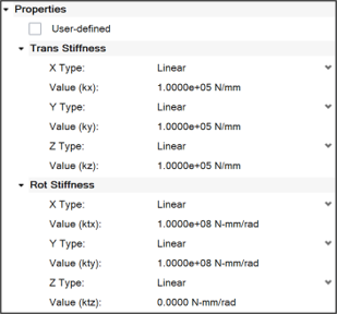
Note: The Z axis of the bushing has been oriented along the axis of the piston pin. Since it is desired to have this bushing behave like a hinge joint, the rotation stiffness about Z axis of the bushing is set to 0.0
-
Change the Rot Stifness value (ktx and kty) to
-
Set the Trans Damping and Rot
Damping properties.
-
Set Value (cx, cy, cz) under Trans Damping to
10 N-sec/mm. -
Set Value (ctx, cty) under Rot Damping to
1000 N-mm-sec/rad.
Figure 10. Damping Properties of Bushing 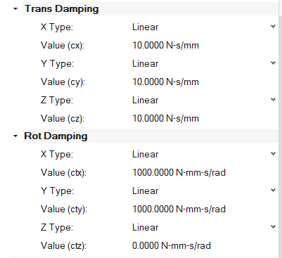
-
Set Value (cx, cy, cz) under Trans Damping to
-
Change the cylindrical Crank-Conrod joint to a Compliant
joint.
Note: Joint compliance is a feature where a rigid joint can be toggled to a bushing and vice-versa. This is a very useful feature to debug potential issues with models having trouble with joints or as a bushing representation.
-
Under the Orientation section, for 1st
Axis:
- Change Align Method to Vector.
- The Vector collector is activated. Hover on the hole surface of the PistonRod to highlight a Vector at its axis and click to create.
Figure 11. Using Hole Surface to Generate Vector for Reference 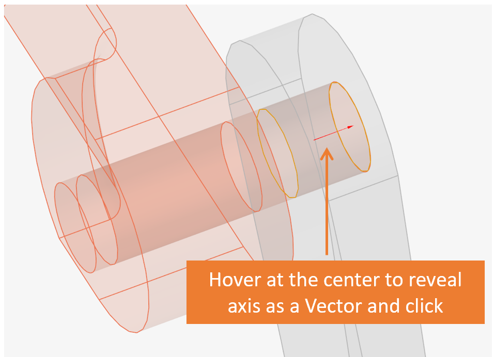
Note: A vector entity Vector 0 is created and resolved into the Vector collector in the compliant joints’ Entity Editor. You may need to rotate and change the model orientation to identify the vector in case the current view does not reveal the vector. -
For the 2nd Axis, retain the Align
Method as DxDyDz change the
Dx, Dy to
0.0and Dz to1.0.Figure 12. Compliant Joint Orientation 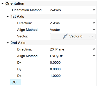
Note: DxDyDz refers to Direction Cosines, a unit vector expressed in terms of Global directions.
-
Under the Orientation section, for 1st
Axis:
Setup Gravity
-
From the Geometry ribbon, under the
Setup group, click on the
Gravity icon
 .
.
-
In the microdialog that appears:
Figure 13. Default Gravity microdialog 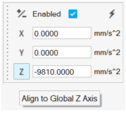
-
Right-click in the modeling window to select
the green check mark and exit the Gravity context.
-
Go to the Analyze Ribbon, click on
Quick Start/Stop Motion Analysis
 to verify that the model behavior has
changed.
The Piston and Conrod should now drop down towards the Crank side.
to verify that the model behavior has
changed.
The Piston and Conrod should now drop down towards the Crank side.
-
Right-click in the modeling window to select
the green check mark
Apply Crank Motion
- can be applied on a joint or on a reference frame (that is, Marker) that belongs to a body.
- can vary with respect to time.
- removes a degree of freedom.
In this model, you will apply a motion on the Crank joint to force the crank to rotate at a certain speed.
-
Go to the Model ribbon, under the
Entities group, click on the
Motions icon
 to enter the Motions context.
- In the guide bar that appears, with the Joint collector active, pick the Crank joint in the modeling window.
-
Click the Create button
 that appears on selecting the joint.
-
Exit the joint context by clicking Cancel
 on the guide bar.
OR
on the guide bar.
ORRight-click in the empty space in the modeling window and click
. -
In the Entity Editor for the Motion just created:
-
Rename the Label and
Varname to
Crank Motionandmot_crankrespectively. - Change the Property to Velocity.
-
Under the Properties section, change the Type to
Expression and Expression
Value to
60d.
Note: Observe the value being evaluated to1.0472rad/s. The “d” is an operator that converts degrees to radians. -
Rename the Label and
Varname to
-
Save
 the Model.
-
Select Default Analysis in the Model Browser and change the End Time to
6. -
Verify the model behavior.
-
Click on the Analysis settings satellite icon
near the Run icon.
-
In the Run Motion Analysis dialog, change the Run
name to
MV_intro2_Motion. - Click Run.
Tip: While building models, it is recommended to add one complexity at a time and verify by solving the model frequently (Crawl-Walk-Run approach) rather than adding all complexities at once and solving it at the end. -
Click on the Analysis settings satellite icon
Add Outputs
-
From the Analyze ribbon, click on the
Outputs icon
 under the Solution group.
-
In the guide bar that appears:
-
Retain Global Frame as the reference frame.
Figure 14. Output guide bar 
-
Click Create
and
 to finish and Exit.
-
Retain Global Frame as the reference frame.
-
Select the output from the Model Browser and change its
Label and Varname to
Crank Displacementando_crank_disprespectively.Similarly, add another output to measure the displacement of the piston using the following choices on the guide bar:- Type: Displacement, Entity, Body
- Body Collector: Piston
- Reference Marker: Global Frame
- Label:
Piston Displacement - Varname:
o_piston_disp
Run Model and Review Outputs
- Run the model using the Run icon.
- Once the run is complete, click Plot in the Run Status dialog.
-
In the HyperGraph page, Create Curve by Files
dialog (Y Source Tab), select the following:
- Types: Marker Displacement
- Requests: Crank on Bearing (Crank Displacement)
- Components: YAW
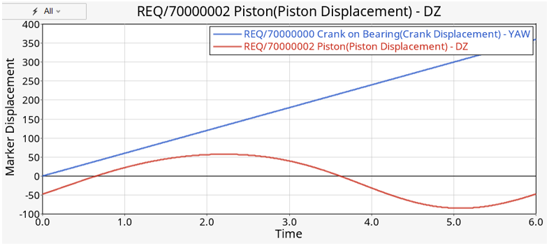
Figure 15. Crank Displacement Output 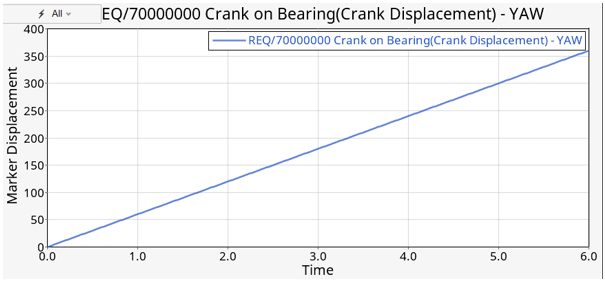
Note: YAW is the component that holds rotational displacement about Z axis. The graph shows crank displacement changing from 0 to 360 degrees in 6 seconds. -
Similarly, plot the piston displacement using the following choices:
- Types: Marker Displacement
- Requests: Piston (Piston Displacement)
- Components: DZ
Figure 16. Piston Displacement Output