Frequency Response Analysis using MotionSolve and Compose
This is an extension of tutorial - MV-2050: Linear Analysis for Stability and Vibration Analysis.
Control system design becomes computationally simpler using mathematical tools like transfer function that can only be applied on Linear time-invariant systems (LTI systems). Linear systems have outputs as a linear combination of inputs. A wide range of physical systems can be approximated very accurately by LTI models.
A Linear Time Invariant (LTI) system in the state space form is described as follows:

where A, B, C, and D are the state matrices, x is the state vector, u is the input vector, and y is the output vector.
MotionSolve can linearize a multibody system by calculating the state matrices for a given set of inputs and outputs through a linear analysis. The states are chosen automatically by MotionSolve.
Frequency response concepts and techniques play an important role in control system design and analysis. In frequency-response methods, we vary the frequency of the input signal over a certain range and study the resulting response.
In this tutorial, you will learn how to convert a multibody model to its equivalent state space form using MotionSolve and obtain corresponding A, B, C, and D matrices. These state space matrices will be further used to construct an equivalent LTI system of the multibody model within Altair’s Compose. Next, a frequency response analysis will be performed on the LTI system using Compose by plotting a Bode Plot diagram.
Next, you can then perform control system design using a variety of tools available within Compose, however this is out of the scope of this tutorial.
- Files Required
-
Before you begin, copy the file(s) used in this tutorial to your working directory.
Review the Model
-
Click
 and open the model
SimplifiedTwoSpring_LTI_START.mdl in MotionView.
and open the model
SimplifiedTwoSpring_LTI_START.mdl in MotionView.
-
Review the simplified model.
The Model contains:
- Two bodies that represent the suspension and bus body.
- Two springs connecting the bus, suspension, and the road.
Figure 1. Simplified Bus Model With No External Disturbance 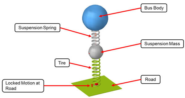
Now, consider a hypothetical force (obtained from a controller) that acts on suspension mass in order to improve the response of system (in other words, bus body displacement) under the effect of disturbance from the road. A simplified block diagram of such a system showing its input and output is shown below.Figure 2. Plant Input - Control Force 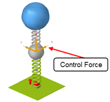
Figure 3. Block Diagram of Plant Showing its Input and Output 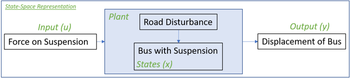
-
The model contains following analyses:
- Transient analysis consisting of a force and a motion.
- Linear analysis consisting of a motion.
In the next step you will perform a transient analysis to identify the output of plant corresponding to a unit value of input.
Transient Analysis - Response at First Mode
In the previous tutorial (MV-2050) the first mode of this system was identified at 1.63Hz (~10.24 rad/s). In this step you will identify the response of this system (in other words, Displacement of Bus) when a unit force is applied at a forcing frequency of 10.24rad/s at Suspension Body.
-
Review the force.
Figure 4. Model with Transient Analysis at Forcing Frequency of First Mode 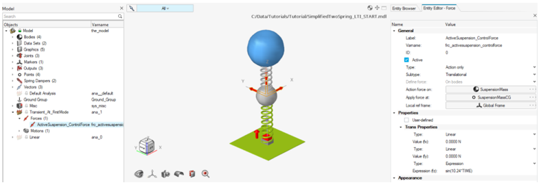
- Review the displacement motion (external disturbance to the plant) at Road, which is currently locked.
-
Run the model.
- From Model Browser, click on the Transient_At_FirstMode Analysis and ensure Analysis Type is set to Static+Transient.
- Go to the Run Motion Analysis window
 .
. - Change the Run name to SimplifiedTwoSpring_Trans and select your <working directory> to output the files.
- Verify that Run active analysis is chosen and
Transient_At_FirstMode is
selected.
OR
Choose the Select analysis option and select the Transient_At_FirstMode analysis.
- Click Run.
Figure 5. Run Motion Analysis Dialog Selections 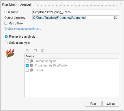
-
Review the results in HyperGraph and plot the
displacement output of BusBody in the vertical direction (Z axis).
Figure 6. Plot Settings for Output Response 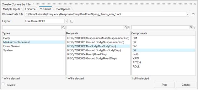
Figure 7. Amplitude of BusBody Displacement for Transient Run 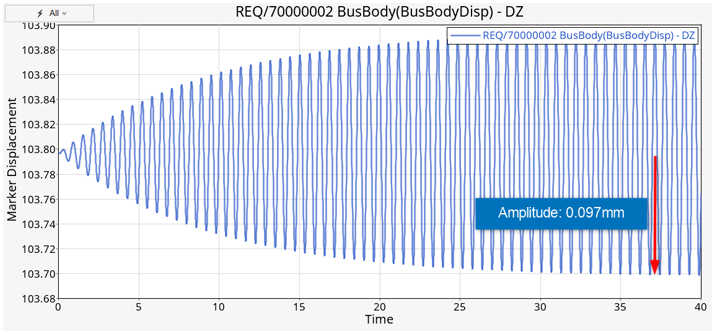
Linear Analysis - Plant Input
In this step you will setup the input of the plant (u). A control force will be applied on the Suspension Mass.
-
Activate analysis Linear Analysis in the model by
right-clicking on Linear in the Model Browser and then selecting Activate > Selected
only.
Note: Review the existing motion in the analysis. An external disturbance is modelled as displacement motion at Road which is currently locked (in other words, zero displacement) to avoid transient conditions.
Figure 8. Activation of Linear Analysis 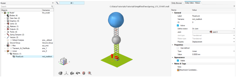
-
Add a SolverVariable to the analysis Linear Analysis
that can obtain the input from the controller to the plant.
- From the Model Browser, click
Linear analysis, select
Model from the Ribbon and click on the
Variables icon in the References group.The Add SolverVariable dialog is displayed.
Figure 9. Add SolverVariable to Represent an Input Port for the Plant 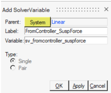
- Change the Label to
FromController_SuspForce. Leave the definition as the default.
- From the Model Browser, click
Linear analysis, select
Model from the Ribbon and click on the
Variables icon in the References group.
-
Add a Solver Array to the analysis Linear Analysis to
define input to the plant.
- From the Model Browser, click
Linear analysis. Then, select
Model from the Ribbon and click on the
References group arrow to invoke additional options. Click on
Arrays.The Add SolverArray dialog is displayed.
Figure 10. Add SolverArray for Plant Input 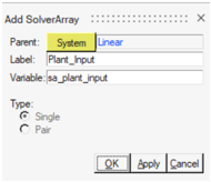
- Change the Label to
Plant_Inputand click OK. - Change the Array type to Plant Input in the
Entity Editor.
Figure 11. Details of the Plant Input 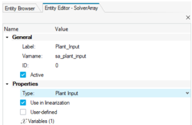
- To choose the SolverVariable as
FromController_SuspForce, click on the
Variables option, select the solver variable
and click on the plus sign
 . Click Apply to
complete the selection.
. Click Apply to
complete the selection. - Activate the Use in linearization check box.
Figure 12. Add a Solver Variable to Plant Input Solver Array 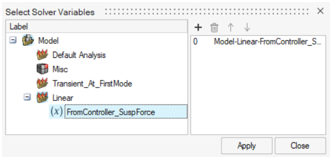
- From the Model Browser, click
Linear analysis. Then, select
Model from the Ribbon and click on the
References group arrow to invoke additional options. Click on
Arrays.
-
Add a force.
- From the Model Browser, click
Linear analysis, select
Model from the Ribbon and click on the
Forces icon
 .
.The Add Force guide bar is displayed.
- Ensure Translational property and Action Only Force are selected.
- Pick SuspensionMass as the Body.Note: Click the ellipsis button
 near the Body
collector on the guide bar to invoke the
advanced entity selector dialog and clear the Only show
entities within valid scope check box to be able to
choose the SuspensionMass body which is outside the
Analysis.
near the Body
collector on the guide bar to invoke the
advanced entity selector dialog and clear the Only show
entities within valid scope check box to be able to
choose the SuspensionMass body which is outside the
Analysis. - Choose SuspensionMassCG as the point of
application of the force and click on the pop-up
Create button
 .
. - From Entity Editor – Force, change Label and
Varname to
ActiveSuspension_ControlForceandfrc_ActiveSuspension_ControlForcerespectively. - In the Tran Properties tab, change
fz to Expression and
set it to
`{sv_fromcontroller_suspforce.VARVAL}`. Hit the Enter key to finish editing.Note: The Expression Builder can be used to create this expression.Figure 13. Forces Guide Bar 
Figure 14. Force Definition 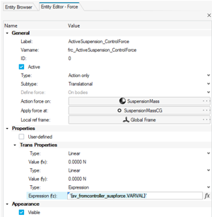
Note: The input from the controller as defined by the solver variable will now be used by the force entity as described by the expression. - From the Model Browser, click
Linear analysis, select
Model from the Ribbon and click on the
Forces icon
Linear Analysis - Plant Output
In this step you will set up the output of the plant (y). A solver variable and solver array will be added to the Linear Analysis in a similar way shown in Step #3 above.
-
Add another SolverVariable with a Label of
FromPlant_BusDisplacementand Varnamesv_fromplant_busdisplacementthat can hold the output from the plant. -
Change the Type to Expression and set its value to
`DZ({b_busbody.cm.idstring})`.Figure 15. Edit SolverVariable to Specify BusBody Displacement 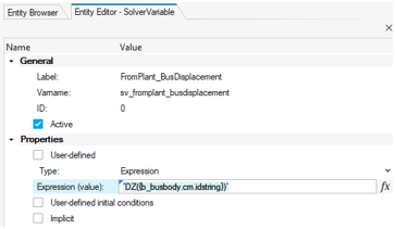
-
Add a Solver Array with a Label of
Plant_Outputto define the output to the plant.- Change the Array type to Plant Output.
- Choose the SolverVariable as FromPlant_BusDisplacement using the collector.
- Select the Use in linearization check box.
Figure 16. Details of the Plant Output 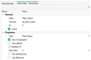
- Save the model as SimplifiedTwoSpring_LTI.mdl.
Set Up and Run a Linear Analysis
-
Set up the analysis type.
- Click on Linear analysis in the Model Browser and set Analysis Type to Static+Linear in the Entity Editor.
- Open the Run Motion Analysis dialog and select the Run offline option.
- Rename the Run name to SimplifiedTwoSpring_LTI.
- Set Analysis to Linear.
Figure 17. Run Motion Analysis Settings 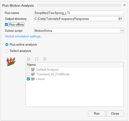
-
Set up the simulation settings.
- Click on the Global simulation settings... button.
- In Analysis Settings, choose the Linear tab from the dialog.
- Ensure that the Altair Compose/Twin Activate OML option from the Generate State Space Matrix group is selected.
- Verify that the Eigen Values And Vectors option check box is cleared.
Figure 18. Simulation Settings 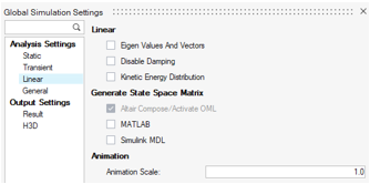
-
Set up the Output Settings.
- In the Output Settings section, click on the Result tab.
- Under Debug Options, activate the Write Debug
Info check box.This will list the states chosen by MotionSolve in the solver log window.
Figure 19. Output Options 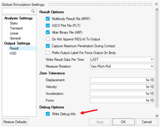
- Click on the Run button to start the simulation.
-
Once the run is complete, review the solver window and observe two independent
coordinates chosen for defining states for the system by MotionSolve (in other words, Translation in Z for BusBody
and SuspensionMass respectively).
Figure 20. Solver Log Window 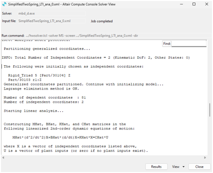
- Observe the run directory and find the Compose script SimplifiedTwoSpring_LTI.oml written out by MotionSolve consisting of the A,B,C, and D matrices.
Frequency Response Analysis in Compose
In this step you will perform a frequency response analysis in Compose using the state space model from MotionSolve. Note that the during the run, an input signal of varying frequencies is supplied to the LTI system and due to its property, the magnitude and phase of the output signal changes while the frequencies itself remain the same.
-
Open Altair Compose and open the oml script
SimplifiedTwoSpring_LTI_ana_0.oml.
- Review the A,B,C, and D matrices.
- Observe the four states listed for the system.
Two states, namely displacement and velocity, are derived from each independent coordinate as described in the MotionSolve solver window.
Figure 21. Review the OML File 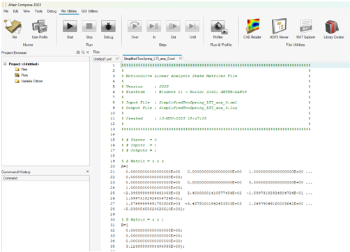
-
Copy and paste the following lines of code:
%Construct a state-space model
SYS=ss(A, B, C, D);

%Construct a transfer function model
%SM_TF=tf(SYS);

%Plot a Bode Diagram
%bode(SYS,R);

%Create a row vector with logarithmically spaced 1000 elements for defining Frequency on X axis
R=logspace(-1, 3, 1000);

%Obtain magnitude and phase response of system using Bode Diagram
[mag,phase]=bode(SYS,R);

%Set up first plot to show magnitude vs frequency using subplot function
subplot(2, 1, 1);
%Set the title for the plot
title('Frequency Response Plot');
hold on;
grid;
%Plot 'mag' in 2D axes with log scale 'R'
semilogx(R,mag);
%Annotate the x and y axes
hx=xlabel('Frequency [rad/s]');
hy=ylabel('Magnitude: BusBody Disp [mm] / Control Force [N]');

%Set up second plot to show phase vs frequency using subplot function
subplot(2, 1, 2);
hold on;
grid;
%Plot 'phase' in 2D axes with log scale 'R'
semilogx(R,phase);
%Annotate the x and y axes
hx=xlabel('Frequency [rad/s]');
hy=ylabel('Phase [deg]');
Figure 22. Insert Code Location 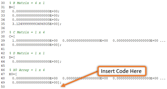
Note: ‘%’ symbol at the start of a line indicates a comment. Review the comments and refer to the Compose documentation for further details. Creating a transfer function is commented out since it is not required for this tutorial. The Default Bode diagram function is also not used here since it uses the decibel scale that is not suitable for this application. -
Run the script by clicking the Start
 button.
-
Observe the variables getting created in the Variable Browser.
Figure 23. Variable Browser 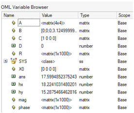
-
Check the figure showing the variation of magnitude and phase of the input
signal as a system response over a range of frequencies.
Note: Two peaks are observed 10.24 rad/s (1.63Hz) and 59.44 rad/s (9.46Hz) corresponding to the natural frequencies of the system.
Figure 24. Frequency Response Plots 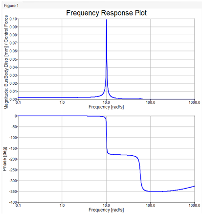
From the Bode Plot one can observe that the amplitude of BusBody displacement per unit force at first mode (10.24 rad/s) would be around 0.098 mm. This output of an approximated linearized model is very close to what we obtained from the MotionSolve transient simulation performed in Step 2. Thus, this linearized model can be further used to perform control system design using Compose.