Quadrotor Control Co-Simulation with Twin Activate
Tutorial Level: Advanced In this tutorial, you will learn how to use MotionSolve and Twin Activate in a co-simulation to control a Quadrotor model.
A quadrotor model is a multirotor helicopter that uses 2 sets of identical fixed pitched propellers (2 clockwise and 2 counter-clockwise) to control lift and torque.
Control of vehicle motion is achieved by altering the rotation rate of one or more rotor discs, thereby changing its torque load and thrust or lift characteristics.
In MotionView you will create the quadrotor frame with 4 superblades and add the rotors motions. A set of forces will be used to represent the wind disturbance.
Twin Activate, through co-simulation with MotionSolve, will implement a controller to impose altitude and direction in quadrotor trying to compensate against the wind effect.
Twin Activate is a software solution for multi-disciplinary, dynamic system modeling and simulation. The software is especially useful for signal-processing and controller design that requires both continuous-time and discrete-time components.
A co-simulation enables MotionSolve and Twin Activate models to communicate with each other during simulation. An ideal use case for co-simulation is the development of a control system for a multibody dynamics model.
Review the Model
- Start a new MotionView session.
-
Select File
Open model
 to load the
Quadrotor_start.mdl file from your working
directory.
to load the
Quadrotor_start.mdl file from your working
directory.
-
Review the model.
The Quadrotor model has 9 bodies, one frame called vehicle, 4 propellers and 4 rotors. Associated with them are their respective graphics.
To connect these 9 bodies there are 4 fixed joints connecting the rotors with the vehicle and 4 revolute joints connecting the propellers with the rotors.
Specify the Propeller's Motion
-
Select the Model Ribbon and click
Motions
 , to display the Motions guide bar.
Figure 1. Motions guide bar 
-
Click on the ellipsis
 next to the Joint collector to access the advanced
selections dialog. Select Propeller_Left and click
OK.
next to the Joint collector to access the advanced
selections dialog. Select Propeller_Left and click
OK.
Figure 2. Select a Joint Dialog 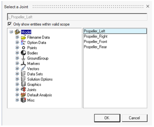
-
Click on the Create icon
 in the Motions microdialog
to add the motion.
in the Motions microdialog
to add the motion.
-
In the Entity Editor, for Label
and Variable, enter
Prop_Left_Rotation and
mot_Prop_Left_Rotation respectively.
Figure 3. Motion's Label and Variable Name in the Entity Editor 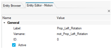
-
In the General section, change the Property to Velocity
and click on
 on the guide bar to finish
editing.
Observe that the guide bar remains open to create new motions.
on the guide bar to finish
editing.
Observe that the guide bar remains open to create new motions.Figure 4. Motion's Property Type Set to Velocity 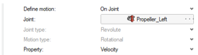
-
Repeat the steps 1-5 to create motion in the other propellers. When complete,
click on the Cancel icon
 to exit the Motions guide bar.
Label Variable On Joint Property Prop_Right_Rotation mot_Prop_Right_Rotation Propeller_Right Velocity Prop_Front_Rotation mot_Prop_Front_Rotation Propeller_Front Velocity Prop_Rear_Rotation mot_Prop_Rear_Rotation Propeller_Rear Velocity In a quadrotor, the velocity of the propeller is defined by the controller of pitch and roll of the vehicle.
To define the velocity value of each propeller motion, create three solver variables in the next step that are used further in the co-simulation.
Specify the Velocity of the Propellers
-
Before you can specify the velocity, you must first create the solver
variables.
-
On the Model tab, click on the Variables icon
 to display the
Add SolverVariable dialog.
to display the
Add SolverVariable dialog.
-
For Variable, enter
sv_Throttle_Command and click
OK.
Figure 5. Add Solver Variable Dialog 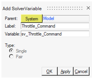
Figure 6. Solver Variable's Entity Editor 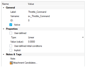
-
On the Model tab, click on the Variables icon
-
Now you can update the propeller motion velocity.
-
From the Properties section, change Type to
Expression and enter:
`VARVAL({sv_Throttle_Command.idstring})+VARVAL({sv_Roll_Command.idstring})`Make sure to hit enter to complete the selection.
Figure 7. Prop_Left_Rotation Motion Expression 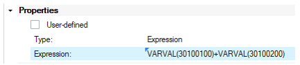
Note: You may need to perform a check model () to get the expression evaluated. -
Repeat the steps above for Propeller Right, Front and Rear, following
the table entries below:
- Motion
- Expression
- Prop_Right_Rotation
-
`VARVAL({sv_Throttle_Command.idstring})-VARVAL({sv_Roll_Command.idstring})` - Prop_Front_Rotation
-
`-VARVAL({sv_Throttle_Command.idstring}) -VARVAL({sv_Pitch_Command.idstring})` - Prop_Rear_Rotation
-
`-VARVAL({sv_Throttle_Command.idstring})+ VARVAL({sv_Pitch_Command.idstring})`
Note: The lateral propellers (left and right) control the Roll of the vehicle and the vertical propellers control the Pitch. The signal difference in the expressions determine the rotation direction of the quadrotor.Figure 8. Propellers' Thrusts To Control the Quadrotor's Motion 
-
From the Properties section, change Type to
Expression and enter:
Add Wind Disturbance Forces
To represent the wind effect and thrust of the quadrotor, a set of forces and moments must be defined.
The wind disturbance is represented as a combination of torques in the X and Y axle applied at the vehicle center.
The thrust of each propeller is represented as a Z force following this equation:
Where,
= Thrust force
= Thrust factor (Defined considering the propeller geometry, air density, m and spin area. For this analysis Tf= 2.1998e-5).
= Propeller Angular velocity
-
Create the wind disturbance force.
-
From the Model ribbon, click on the
Forces icon
 to open the Forces guide bar.
Figure 9. Wind Disturbance Force guide bar 
-
Click on the Create icon
 to generate the Force.
-
In the Entity Editor, enter
Wind_Disturbance for
Label and
frc_Wind_Disturbance for
Varname.
Figure 10. Forces Entity Editor 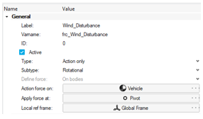
-
From the Rot Properties tab, set
tx and ty to
0.5 and click on
 to exit editing the current Force.
Figure 11. Rotational Properties Section Parameters 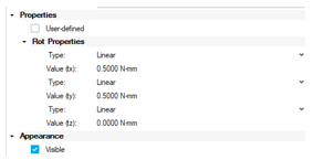
-
From the Model ribbon, click on the
Forces icon
-
Create the thrust force.
-
Click on the Forces icon to open the Forces guide bar.
-
Select Left_Rotor as the Reference
Marker.
Figure 12. Thrust Force guide bar 
-
In the Entity Editor, enter
Thrust_Left for Label
and frc_Thrust_Left for
Varname.
Figure 13. Thrust Force Entity Editor 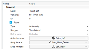
-
From the Trans Properties tab, change fz to
Expression and enter the expression:
`2.1998e-5*ABS({j_Propeller_Left.WZ})^2`.Figure 14. Trans Properties Parameters 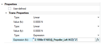
-
Repeat the steps to create the thrust force for the right, front, and
rear rotors.
- Thrust Right
- Label
- Thrust_Right
- Variable
- frc_Thrust_Right
- Body 1
- Rotor_Right
- Origin
- Right_Motor_Center
- Ref Marker
- Right_Rotor
- fz Expression
`2.1998e-5*ABS({j_Propeller_Right.WZ})^2`
Figure 15. Right Rotor's Entity Editor Parameters 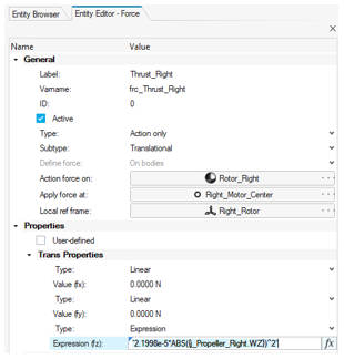
- Thrust Front
- Label
- Thrust_Front
- Variable
- frc_Thrust_Front
- Body
- Rotor_Front
- Point
- Front_Motor_Center
- Ref Marker
- Front_Rotor
- fz Expression
`2.1998e-5*ABS({j_Propeller_Front.WZ})^2`
Figure 16. Front Rotor's Entity Editor Parameters 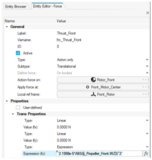
- Thrust Rear
- Label
- Thrust_Rear
- Variable
- frc_Thrust_Rear
- Body
- Rotor_Rear
- Point
- Rear_Motor_Center
- Ref Marker
- Rear_Rotor
- fz Expression
`2.1998e-5*ABS({j_Propeller_Rear.WZ})^2`
Figure 17. Rear Rotor's Entity Editor Parameters 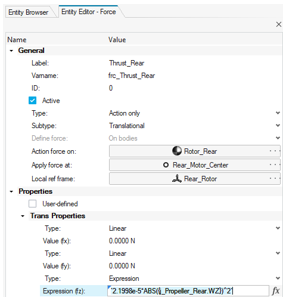
-
Click on the Forces icon
- To save your model, click Save As and save it with the name Quadrotor_tutorial.mdl.
Create Control Inputs and Plant Outputs
To modify the MBS model to work in a Co-Simulation Mode you need to add solver arrays and solver variables entities in MotionView model. The solver variables contain the individual plant input and output values. The solver arrays define the plant input and output to communicate with Twin Activate.
-
Adding solver variables.
- The individual plant input solver variables were already defined with the propellers motion in Specify the Velocity of the Propellers. They are Throttle_Command, Roll_Command and Pitch_Command.
-
Next, you will define the individual plant output values, which are Altitude,
Roll Angle, Pitch Angle, X position, Y position, X velocity and Y
velocity.
-
In the Model ribbon, click on the
Variables icon
 in the References
group, to open the Add SolverVariable dialog and
add the following solver variables:
in the References
group, to open the Add SolverVariable dialog and
add the following solver variables:
Label Variable Expression Altitude sv_Altitude `DZ({m_Vehicle.idstring})`Roll_Angle sv_Roll_Angle `AY({m_Vehicle.idstring})`Pitch_Angle sv_Pitch_Angle `AX({m_Vehicle.idstring})`PosX sv_PosX `DX({m_Vehicle.idstring})`PosY sv_PosY `DY({m_Vehicle.idstring})`VX sv_VX `VX({m_Vehicle.idstring})`VY sv_VY `VY({m_Vehicle.idstring})`Note: Remember to set the Type in the SolverVariable Properties tab to Expression.
-
In the Model ribbon, click on the
Variables icon
-
Create two solver arrays, ControlInput and PlantOutput, to communicate with
Twin Activate.
-
In the Model ribbon →
References group, click on the arrow to
expand additional options. Click on Arrays to
open the Add SolverArray dialog.
Figure 18. Solver Arrays Icon 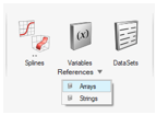
Tip: You can use the search field located in the top right corner of the window to search for any functionality, for example Array in this case. -
From the Properties section, change the Array
type to Plant Input.
Figure 19. Solver Array Type set to Plant Input 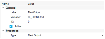
-
Click on Variables
 in the Entity Editor, to invoke the Select a Solver dialog.
-
Select Roll_Command for SolverVariable 0,
Throttle_Command for SolverVariable 1 and
Pitch_Command for SolverVariable 2 in this
order. To add entities, first click on the Solver Variable on the left
and then on the plus sign on the right. Finally, click the
Apply button to complete the Solver Array
creation.
Figure 20. Plant Input Variables 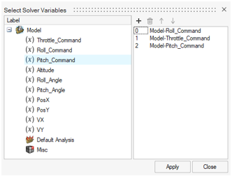
-
From the Properties tab, change the Array type
to Plant Output.
Figure 21. Solver Array Type set to Plant Output 
-
Select the Roll_Angle,
Altitude, Pitch_Angle,
PosX, PosY,
VX, and VY variables
in this order and click Apply.
Figure 22. Plant Output Variables 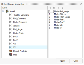
-
In the Model ribbon →
References group, click on the arrow to
expand additional options. Click on Arrays to
open the Add SolverArray dialog.
-
Save your model
 .
.
Run the MBS Model in MotionSolve for Verification
-
From the Analyze ribbon, click on Analysis settings
 next to Run, to open the Run
Motion Analysis dialog.
next to Run, to open the Run
Motion Analysis dialog.
- Select the Run offline option.
- Rename the Run name input to Quadrotor_tutorial.
- Select an Output directory folder, where the results will be save and click on the Run button.
Figure 23. Run Motion Analysis Window 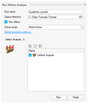
-
Click Results to animate the simulation results and
confirm that the model works as intended before continuing to the next
step.
Note: The controller is not yet connected to the model, so the input force and torque are zero.
Connect MotionSolve with Twin Activate
- From the All Programs menu, launch Twin Activate.
-
From the menu bar, select
 to load the Quadrotor_Control_Start
.scm file from your working
directory.
to load the Quadrotor_Control_Start
.scm file from your working
directory.
-
Review the model.
The system has 3 sections of control: Altitude of the quadrotor, X position and Y position. The X and Y position control is defined by a target path, for this model it is a slope of 0.025.
Figure 24. System’s Three Control Sections 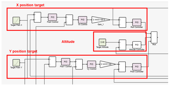
These three sections of controls defined by seven PIDs are the plant input for the MBS model. In MotionView, it's defined as Roll_Command, Throttle_Command and Pitch_Command.
The plant output, Roll_Angle, Altitude, Pitch_Angle, PosX, PosY, VX, and VY, are input for the PID controls.
For example, in the X position target control, you will see three inputs which come from the plant output (PosX, VX, and Roll Angle).Figure 25. X Position Target Control Section 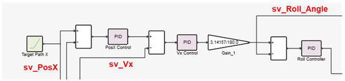
-
To enable co-simulation between Twin Activate and
MotionSolve, from Twin Activate, select . In the dialog that is displayed, define the MotionSolve and MotionView
license paths.
Figure 26. Twin Activate Preferences 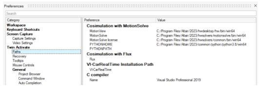
-
From the Palette Browser, select , and drag-and-drop the MotionSolve
block into the current diagram and connect the blocks.
Figure 27. MotionSolve Block Inclusion 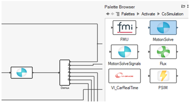
-
From the diagram, double-click the MotionSolve block. From the dialog that
is displayed, define the following block properties:
The following parameters are populated automatically after you load the input model, *.mdl or *.xml:
- Inputs Row Size: The value 3 indicates that three signals are supplied from Twin Activate to the MotionSolve model. These signals correspond to the solver array PlantInput, with variables Roll_Command, Throttle_Command and Pitch_Command.
- Outputs Row Size: The value 7 indicates that the MotionSolve model is sending out seven signals
from one port, which is why the Demux block is added to separate the
signals. The signals correspond to the solver array PlantOutput with
variables Roll_Angle, Altitude, Pitch_Angle, PosX, PosY, VX and VY.
Figure 28. MotionSolve Loaded Model’s Parameters Ribbon 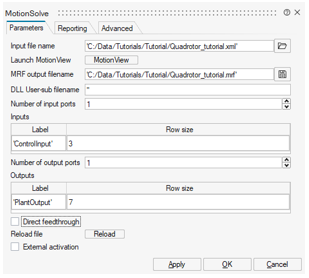
Figure 29. MotionSolve Loaded Model’s Advanced Ribbon 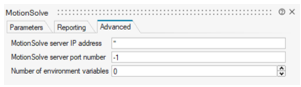
Co-simulation with Twin Activate can be done in two ways:- Local co-simulation
- In this case, both MotionSolve and Twin Activate are installed on the same machine. You do not need any additional setup and the fields “MotionSolve server IP address” and “MotionSolve server port number” can be left at their default values as shown in the figure above. Upon starting the co-simulation from Twin Activate, the connection between the two solvers is made automatically, based on the paths specified in Step 4.
- Remote co-simulation between Twin Activate and MotionSolve
- In this case, MotionSolve and Twin Activate can be located on different machines that are accessible over the network. The following section describes how remote co-simulation can be accomplished.
To co-simulate, continue following the rest of this tutorial.
-
Click and drag to connect the output of the block Mux to
Control Input of the MS Plant. Similarly, connect the Plant Output end of the MS
Plant to the input end of Dmux. All required blocks are
now present and connected in the modeling window.
Figure 30. Twin Activate Co-simulation Model Diagram 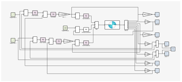
-
From the ribbon's Simulate tool group, select the Setup
 tool. From the
Simulation Parameters dialog, in the Final Time field,
enter 12 so that your simulation runs for twelve
seconds.
tool. From the
Simulation Parameters dialog, in the Final Time field,
enter 12 so that your simulation runs for twelve
seconds.
Figure 31. Simulation Parameters 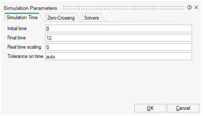
Note: Since Twin Activate is the main, or calling, solver in this co-simulation scenario, if the simulation end time in Twin Activate is different than the MotionSolve simulation end time, the MotionSolve simulation end time will be modified at run time to match the end time specified in the Twin Activate dialog above. -
From the ribbon, click Run
 .
The Scope blocks in the model generate the following plots, which illustrate the altitude, roll, pitch, x position, y position, and the path.
.
The Scope blocks in the model generate the following plots, which illustrate the altitude, roll, pitch, x position, y position, and the path.Figure 32. Altitude 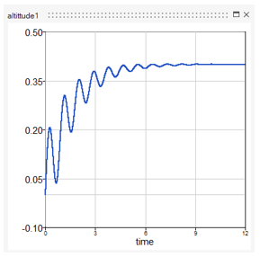
Figure 33. Roll 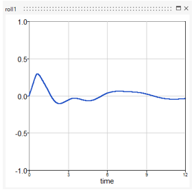
Figure 34. Pitch 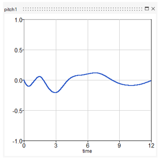
Figure 35. X Position 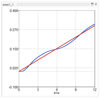
Figure 36. Y Position 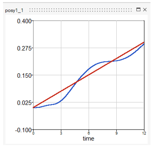
Figure 37. X Velocity 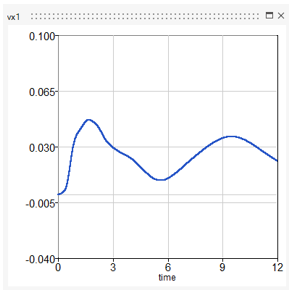
Figure 38. Y Velocity 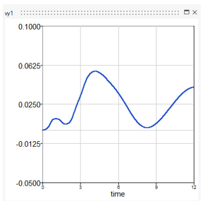
Figure 39. XY Path 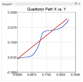
-
Launch HyperView and animate the
Quadrotor_tutorial.h3d file to see the quadrotor
behavior.
Figure 40. Load H3D File in HyperView 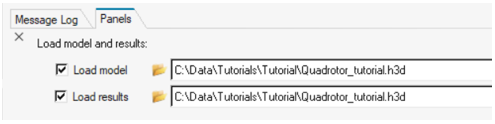
Figure 41. 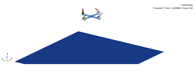
- Before exiting the applications, save your work in Twin Activate as quadrotor_complete.scm.