3D Mesh-to-Mesh Contact Simulation
Tutorial Level: Intermediate In this tutorial, you will learn about 3D rigid body contact capabilities in MotionSolve and use the mesh-to-mesh contact approach, which uses surface meshes for the bodies in contact during the simulation.
- Each mesh component should form a closed volume. This means that the given mesh should not contain any open edges (edge which is part of only one element) or T- connections (2 elements joined at the common edge in the form of a T).
- Mesh should be of uniform size.
- Element surface normal should point in the direction of expected contact.
- Import CAD geometry with graphic settings suitable for contact simulation.
- Setup 3D rigid body contact between meshed geometries in the multibody model.
- Perform a transient analysis to calculate the contact forces between these geometries.
- Post-process the results using a report generated automatically.
For this tutorial, you will use a slotted link model.
For this type of meshed representation of 3D rigid bodies, MotionSolve uses a numerical collision engine that detects penetration between two or more surface meshes and subsequently calculates the penetration depth(s) and the contact force(s).
- Slotted Link Model
-
A slotted link mechanism (sometimes also referred to as a scotch-yoke mechanism) is a type of mechanism used to convert an input rotational motion into continuous or intermittent translational motion of a sliding link or yoke part. The motion is transferred via a contact force between parts of the mechanism that are in contact. Both normal and friction contact force may be responsible for the transfer of motion.
Such mechanisms find common application in valve actuators, air compressors, certain reciprocating and rotary engines, among others. The figure below illustrates a slotted link mechanism that will be modeled in this tutorial.
Figure 1. A Slotted Link Mechanism. The cam is in contact with the slotted link as shown, whereas the pin comes into contact with the slots. 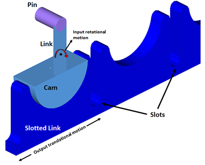
Import CAD Geometry into MotionView
- Start a new MotionView session.
-
From the Menu bar, click and then select Geometry or FEM using HyperMesh.
Figure 2. Invoke Geometry or FEM using HyperMesh Option 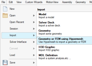
The Import CAD or FE using HyperMesh dialog is displayed. -
Set the following options in the dialog:
-
Click the file browser icon,
 , to navigate to your working directory and
select slotted_link.x_t as the input CAD
geometry.
The Output Graphic File text field is automatically populated with the same path and name, however it is suffixed with a _graphic.h3d extension. This file will be used to specify the graphics in the model. You may change the name or path of the graphic H3D if you prefer.
, to navigate to your working directory and
select slotted_link.x_t as the input CAD
geometry.
The Output Graphic File text field is automatically populated with the same path and name, however it is suffixed with a _graphic.h3d extension. This file will be used to specify the graphics in the model. You may change the name or path of the graphic H3D if you prefer. -
Click
 to expand the Meshing
Options for the Surface Data section. Verify that Allow
HyperMesh to specify mesh
options is selected.
to expand the Meshing
Options for the Surface Data section. Verify that Allow
HyperMesh to specify mesh
options is selected.
-
Activate the Control mesh coarseness for
contacts check box. Set the slider to
5.
Selecting this option instructs HyperMesh to mesh the CAD geometry so it can be used for 3D contact in MotionSolve.Note: The slider controls the coarseness of the generated mesh, with 1 being the coarsest and 10 being the finest. A very coarse mesh has large triangles, which may not represent the curvature of the CAD surfaces accurately. Alternatively, a very fine mesh has extremely small triangles that may increase element numbers and thereby the solution time. The best practice is to strike a balance between mesh fineness and performance that satisfies the modeling purpose.At this stage, the Import CAD or FE using HyperMesh dialog should look like the figure below:
Figure 3. Selections on the Import CAD or FE using HyperMesh Dialog 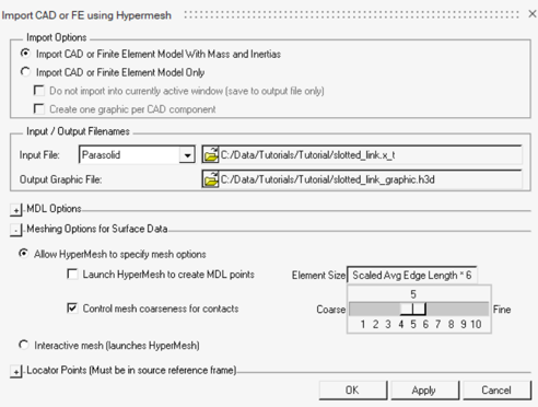
-
Click the file browser icon,
-
Click OK.
MotionView invokes HyperMesh in the background to mesh the geometry and calculate its volume properties. The Import CAD dialog is displayed. From this dialog, you can review the components in the CAD file as well as their mass, density, and volume properties.
Figure 4. CAD Component List on the Import CAD Using the Import CAD or FE Utility Dialog 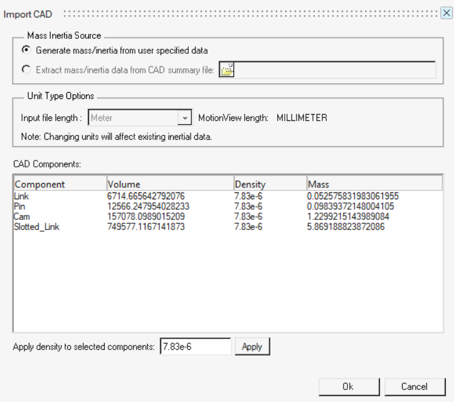
-
Click OK and clear the Message Log.
The converted geometry is loaded into MotionView for visual inspection. You can inspect the surface mesh by swapping the display to a meshed representation.
- From the Model Browser, click on Graphics to open the list of available body graphics.
- Select .
-
In the Entity Editor, click on Mesh > Mesh
Lines
 , then click Apply and
OK.
, then click Apply and
OK.
Figure 5. Displaying Mesh Lines for a Graphic Component of the Input CAD Geometry 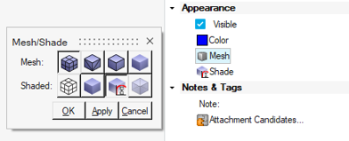
Repeat Steps 7-8 for the rest of the Graphics:- Pin
- Cam
- Slotted_Link
Figure 6. Displaying the Surface Mesh for all Components of the Input CAD Geometry 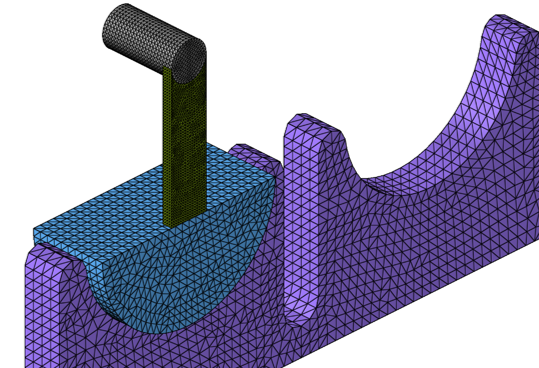
Create Joints and Motion
At this stage, the model contains the following bodies along with their associated graphics:
| Entity name | Entity type | Description |
|---|---|---|
| Slotted_Link | Rigid Body | The slotted link body. |
| Cam | Rigid Body | The cam body. |
| Pin | Rigid Body | The pin body. Together the cam and the pin bodies engage the slotted link. |
| Link | Rigid Body | A connector body between the pin and the cam. |
| Slotted_Link | Graphic | The graphic that represents the slotted link body. This is a tessellated graphic. |
| Cam | Graphic | The graphic that represents the cam body. This is a tessellated graphic. |
| Pin | Graphic | The graphic that represents the pin body. This is a tessellated graphic. |
| Link | Graphic | The graphics that represent the link body. This is a tessellated graphic. |
The Pin, Link, and Cam bodies are fixed to each other and pivoted to the Ground Body at the Cam center. The Slotted_Link can translate with respect to the Ground Body.
-
Create joints,
 , per the details in the table below:
S.No Label Type Body 1 Body 2 Origin Alignment Axis 1 Pin Link Fix Fixed Joint Pin Link Pin CG 2 Link Cam Fix Fixed Joint Link Cam Link CG 3 Cam Pivot Revolute Joint Cam Ground Body Global Origin Global Y 4 Slotted Link Slider Translational Joint Slotted_Link Ground Body Slotted_Link CG Global X -
Apply a motion,
 , on the Cam Pivot joint of the type
Displacement and define the
Expression as
, on the Cam Pivot joint of the type
Displacement and define the
Expression as `360d*TIME`. - Save your model as slotted_link_mech.mdl.
Define Contact Between the Colliding Geometries
- Cam and the Slotted_Link
- Pin and the Slotted_Link
-
From the Model ribbon, click on the
Contacts icon,
 on the Entities toolbar.
The Add Contact guide bar is displayed.
on the Entities toolbar.
The Add Contact guide bar is displayed. - Select 3D for the type of contact.
-
Resolve Body 1 to Cam and Body 2 to
Slotted_Link, and click the
Create button
 . This automatically selects the respective graphics
that are attached to these bodies.
. This automatically selects the respective graphics
that are attached to these bodies.
Figure 7. Contacts guide bar 
-
Change the Label to Cam Slotted
LinkContact.
Note: To properly define the geometries, ensure that the normals are oriented correctly and that there are no open edges or T-connections in the geometries.
-
From the Entity Editor, activate the
Highlight contact side check box. This colors the
geometries specified for this contact force element according to the direction
of the surface normals. Verify that both geometries are completely red (to
visualize clearly, you may have to deactivate the other graphic and
reactivate).
Figure 8. Activate Highlight Contact Side Check Box 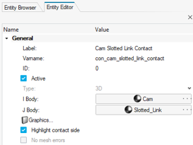
Figure 9. Check for Incorrect Surface Normals 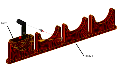
Red indicates the direction of the surface normal and is the side of the expected contact.
-
Check for open edges or T-connections. If the associated graphics mesh has any
open edges or T-connections, the Highlight mesh errors option is active. If it
is active, select the check box for Highlight mesh
errors.
Any open edges or T-connections in the geometry are highlighted.The graphics associated in this contact entity do not have any mesh errors. Therefore, No mesh errors is displayed and grayed out.
Figure 10. 
The geometry is clean; there are no free edges or T-connections in the model.
Note: For every contact entity added to the model, MotionView automatically creates an output, , of the type Expression that
can be used to plot the contact forces for that contact
element.
, of the type Expression that
can be used to plot the contact forces for that contact
element. -
Specify the contact properties. Under the Properties
tab, the Normal Force and the Friction Force property sub-tabs are displayed. In
this model, you will use an Impact model with the following properties:
- Normal Force
- Type
- Impact
- Stiffness
- 1000.0
- Exponent
- 2.1
- Damping
- 0.1
- Penetration Depth
- 0.1
- Friction Force
- Type
- Disabled
Figure 11. Contact Entity Editor - Properties Group 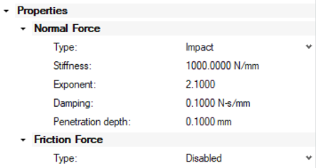
Note: MotionSolve supports several contact methodologies. A more detailed description on each method and their properties can be found at Force: Contact. -
Change the location where contact forces are applied to a surface mesh.
- Select the Advanced tab.
- From the Force Computed at drop-down menu, select Node.
Figure 12. Change the Location Where the Nodes are Computed 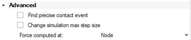
Note: By default, contact forces are resolved at the center of each element of the surface mesh. This setting is satisfactory in most contact applications. However, you can force MotionSolve to apply the contact forces on the nodes of the surface mesh instead. This is useful in cases where a geometric edge is in contact but comes with a slight penalty in computational performance. - Repeat Steps 1 - 8 for creating contact between the Pin body (Body I) and the Slotted_Link (Body J). You may define the label for this contact to be Pin Slotted Link Contact. Define the same contact properties as listed in Step 8 above.
-
For the contact force element Pin Slotted Link Contact, you will also instruct
MotionSolve to find the precise time at which
contact first occurs between the two colliding bodies.
-
In the text field below, for Max step size scale factor, specify a
value of 0.01.
Figure 13. Contact Entity Editor - Advanced Group 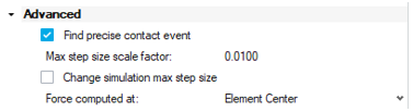
Note: With the Find precise contact event option, MotionView automatically adds a sensor entity (defined by Sensor_Event in the solver deck), which has a zero_crossing attribute. During simulation, when the contact force is detected for the first time (force value crossing zero), MotionSolve reduces its step size by the given factor and attempts to determine the contact event more precisely.
-
In the text field below, for Max step size scale factor, specify a
value of 0.01.
Set Up a Transient Simulation and Run the Model
At this point, you are ready to set up a transient analysis for this model.
- From the Model Browser, click Default Analysis, to display its Entity Editor.
- Navigate to the Analysis Parameters group and verify that the Simulation type is set to Transient and specify an end time of 3.0 seconds.
-
To obtain accurate results, specify a smaller step size than the default. Go to
the Dynamic Settings group and set the Maximum Step Size
to 1e-3.
Figure 14. Specifying the Maximum Step Size 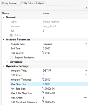
- From the Analyze ribbon, click on Analysis Settings next to the Run icon to open Run Motion Analysis dialog.
-
Select the Run Offline option, specify a Run name and a
directory where the results will be written, and click
Run.
The transient simulation is started.
Figure 15. Specify the Output File Name and Run the Model 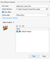
The HyperWorks Solver View dialog displays a message from the solver that confirms that the mesh-based contact method is being used for the contact calculations.Figure 16. Verifying Mesh-Based Contact is Used for the Simulation 
The log file contains messages related to the sensor. This is a result of finding the precise contact event for the second contact element in the model.Figure 17. Solver Message Related to Sensor Activity 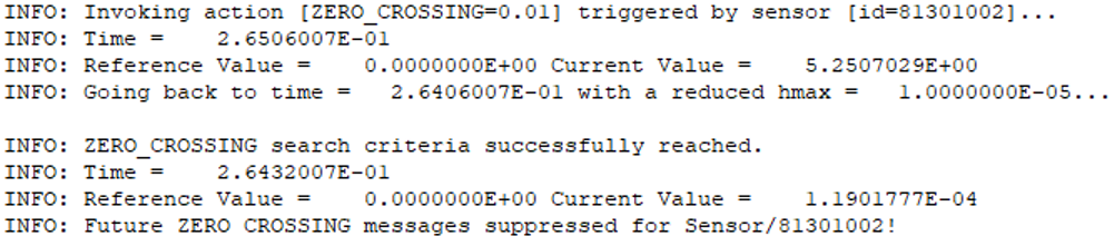
Post-process the Results
- Close the solver window.
-
To view a consolidated report of the results, click on the
AnalyzeRibbon and select
Reports
 .
A list of previous simulations you have completed using MotionView is displayed.
.
A list of previous simulations you have completed using MotionView is displayed. - Select the Contact Report that corresponds to this simulation.
-
Click OK.
Figure 19. Create Contact Report 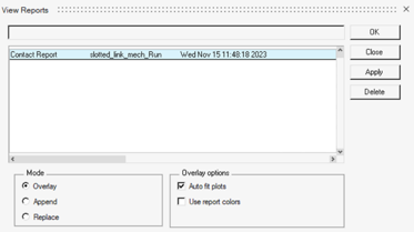
MotionView creates several pages in your current session.
Visualize the Contact Forces via H3D
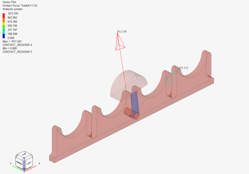
The first HyperView page (second in the session) displays a vector animation of contact force aggregated over the contact region. You may hide one or more parts to view this clearly in the modeling window. This is illustrated in the figure below.
Contact Summary
Use the Page Navigation icon, ![]() , to navigate to the next page.
, to navigate to the next page.
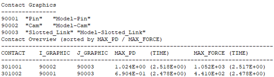
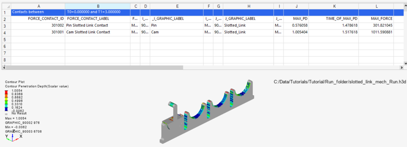
The third page in the session can be used to get an overall summary of the contact simulation. This page contains table that tabulates the summary, as well as a HyperView window that displays the penetration for the entire simulation. The table provides a summary of the maximum penetration depth and maximum force. This page provides a bird’s eye view of the contact phenomenon happening within the model. The contour of penetration depth is a static image that highlights all regions that come under contact during the entire period of the simulation.
Visualize the Penetration Depth via H3D
Navigate to the next page.
The fourth page in the session (HyperView) can be used to visualize the penetration depth over the course of the simulation.
-
Click the Start/Pause Animation icon,
 , to animate the result.
-
Set the graphic display to Transparent Elements and
Feature Lines.
Figure 22. Set Display to Transparent Elements and Feature Lines 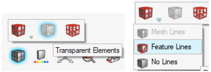
The animation is shown in the figure below:Figure 23. Penetration between the Cam Body and the Slotted Link 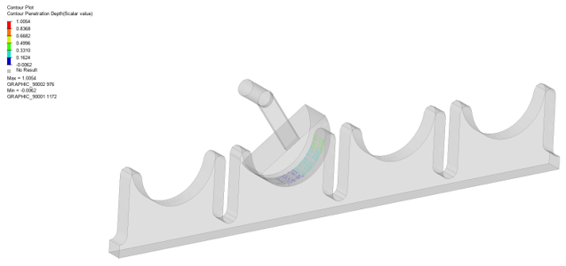
Visualize MotionSolve Outputs
-
Navigate to the Vector panel,
 .
.
-
For the Result type, select the result type from the drop-down menu and click
Apply.
This plots the result type you selected for all relevant graphics in the model. You may have to scale the force vectors accordingly to make sure they are visible.
Figure 24. Scaling the Tangential Force 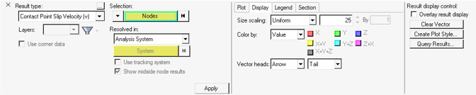
For example, the point slip velocity vectors are plotted in the figure below:Figure 25. Point Slip Velocity Vectors 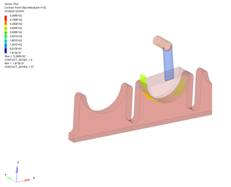
Plot the Contact Forces via ABF
Manually Plot Other Output Requests
-
Click Add Page, and change the client to , (if it is not already selected).
Figure 27. Add a Page 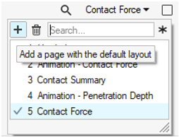
-
Open
 the ABF output file for the
simulated model.
the ABF output file for the
simulated model.
-
Under Y Source, select Type as
Expressions and select a request in the Requests
window.
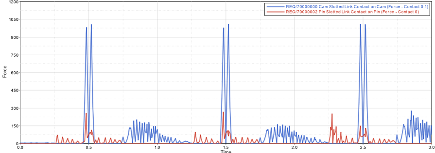
Select REQ/70000003 Pin Slotted Link Contact on Slotted_Link (Force – Pin Slotted Link Contact) as the Request and F4 as the Component to plot.
Figure 28. Open ABF File and Select the Requested Output 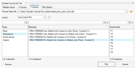
-
Click Plot.
Figure 29. Visualizing the Contact Force in HyperGraph 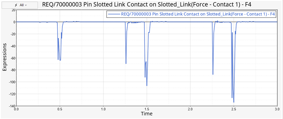
- Save your session as slotted_link.mvw.
Summary
In this tutorial, you learned how to create a well-meshed representation from CAD geometry. Further, you learned how to set up contact between meshed geometries. Also, you were able to inspect the geometry to make sure the surface normals were correct and there were no open edges or T connections.
You were also able to setup a transient analysis to calculate the contact forces between these geometries and post-process the results via vector and contour plots, in addition to plotting the contact force requests.