Introduction to MotionView - Part 1
Tutorial Level: Beginner This tutorial will help users who are new to Multi-body modeling become familiar with the MotionView interface and the process of model building, solution, and results review.
- Invoke MotionView
- Import CAD Geometry
- Set up the Model
- Solve the Model
- Review the Results
Invoke MotionView
In this step, you will learn how to invoke MotionView.
-
In Windows, click Start Menu
 > Altair <version> >
  MotionView
<version> OR using the Altair ConnectMe app (if installed).
Once invoked, the launcher window appears as shown in the image below.
MotionView
<version> OR using the Altair ConnectMe app (if installed).
Once invoked, the launcher window appears as shown in the image below.Figure 1. Launcher Window 
- Select MotionView and create a new session.
-
In Linux, invoke
~hw_install/altair/scripts/mviewin an open terminal (where~hw_installis the location of the installation).
- The MotionView Interface
-
A new session is launched with a page/window displaying MotionView as the active client.Note: A session can consist of one or more pages. Each page can have multiple window layouts, with each window having a different client serving different modeling and result review needs. The following clients are available:
- HyperGraph - Plotting
- HyperMesh - Finite Element Modeling
- HyperView - Animation
- MotionView - Multibody Modeling
- TableView - Table Processing
- TextView - Text Processing
Figure 2. Interface Elements 
MotionView is organized into these various areas:- The Title Bar displays the name of the session file as well as the active product version.
- The Menu Bar provides access to Ribbons, standard functions such as file management operations, system preferences, help, and configuring the visibility of various areas of the interface. You can also change the active product from the menu bar.
- The Pages and Windows can be changed to control the main display area. Each page can have up to 16 windows.
- The Search allows you to quickly find various tools and functionalities that are also available from the ribbons.
- The Ribbon allows you to quickly access tools and standard functions and is located along the top of MotionView. Click on an icon to open the related tool. Hovering over a group of icons may reveal additional tools.
- The Model Browser lists various entities of a model in a tree-based format. A context sensitive menu allows you to perform various actions like copy/paste, hide/show, and so on, on each node of the tree.
- The Entity Editor lists all the properties of the selected entity.
- The Modeling Window displays the model while it is being setup, as well as animates the same during a solver run (MotionSolve only) and results review. This also contains other interactive areas like the Guide Bar, Microdialog, Toolbelt, and Entity Selection Filter.
- The Client Window allows you to work with other clients like HyperGraph, HyperView, and so on, side by side.
- The Status Bar about the currently loaded model and lists the status of MotionView at any point of time like Ready, Importing Geometry, and so on.
- The View Controls allows you to control the view and display of the model in the modeling window.
- The Animation Controls allows you to review the animation of a model after a run.
Import CAD Geometry
In this step, you will learn how to import a CAD geometry file in MotionView.
-
Observe the default contents of the model from the Model Browser.
Figure 3. Model Browser 
Note: Each entity folder in Model Browser can be expanded or collapsed to see its content and has a count of entities contained in the same within the () parenthesis. For example, there is a Ground Body by default in the Bodies folder. Ground Body does not move during a simulation. -
Import the CAD geometry using one of the following methods:
- Drag and drop PistonCylinderAssembly.x_t from your working directory into the modeling window of the MotionView client.
- From the Menu Bar, click , select PistonCylinderAssembly.x_t, and click Open.
The geometry is imported.Figure 4. Imported CAD Geometry 
Observe the Model Browser. It shows eight Bodies (other than Ground Body) and eight Graphics entities. When a geometry is imported, each CAD component is represented with a Body entity and a corresponding Graphic entity of type CADGraphics.- A Body entity represents mass and inertia.
- A Graphic entity is a geometrical object used for visualization and while solving a contact problem.
-
Use the following mouse controls to manipulate your model in the modeling window:
- Pan the model by holding down the right mouse button while dragging the mouse.
- To Rotate, hold down the middle mouse (or Shift + right mouse) button while dragging the mouse.
- Use the scroll wheel to Zoom centered on the mouse cursor.
-
In the modeling window hover on the
Piston (component in green in the image below). The
object is highlighted along with the object label appearing in a bubble text.
Click on the object and notice that the body gets selected.
Figure 5. Picking from the Modeling Window 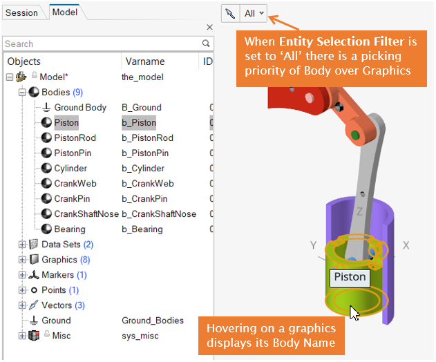
-
Change the Entity Selection filter (available on the top
left of the modeling window) from
All to Graphics and again
click the same “Piston” object on the screen.
Figure 6. Using Entity Selection Filter 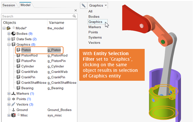
Note: This time the Graphics entity has been selected (indicated in the Model Browser). - Double-click the empty space in the modeling window to deselect everything.
- Revert the Entity Selection filter to All.
Set up the Model
In this step, you will learn how to set up your model.
-
Ground the Bearing and Cylinder bodies.
-
Select the Bearing and
Cylinder bodies.
Note: The selected bodies are highlighted in red. Also, the Model Browser now shows these bodies with a grounded icon
 .
. -
Right-click in an empty space and select the green check mark
 to exit the Ground Context.
Figure 7. Grounding Bodies from Ground Group Context 
Note:- Using a Ground Context can be useful when there are multiple bodies to be grounded or un-grounded.
- A body can also be grounded using the Ground option in the right-click context menu of the body.
- Observe the Ground Group in the Model Browser. Selecting this group highlights all the bodies that have been grounded.
- When a body is grounded, the entities that have the grounded body as a parent are moved to the Ground Body during solution.
-
Select the Bearing and
Cylinder bodies.
-
Set up the PistonHead Rigid Group.
A Rigid Group is a collection of bodies that are assumed to be rigidly connected with each other. The concept is like Ground Group, except that a Rigid Group is collectively represented and treated as one rigid body during solution.
-
Click the ‘Group’ button available on the
microdialog to create a Rigid Group with the
selected bodies.
Figure 8. Creating a Rigid Group 
Note: The newly created Rigid Group with a default name ‘RigidGroup 0’ is visible in the Model Browser. -
Change the RigidGroup’s label from ‘RigidGroup 0’ to
‘PistonHead’ using the Entity Editor.
Alternatively, the renaming can also be done by right-clicking on the object in the Model Browser and using Change Label (keyboard shortcut F2).
Figure 9. Editing Properties using the Entity Editor 
Figure 10. Using the Model Browser to Rename 
Note: The Entity Editor shows all the properties of the selected entity. The same can be used to quickly edit properties. Currently, there are Panels in the bottom area of the window that exist in the legacy MotionView interface which are used to edit the same properties. In future releases, the Panels will be removed and will be replaced by Entity Editors.Click the green check mark on the guide bar to Finish
Editing.
on the guide bar to Finish
Editing.The context is again in 'Create' mode.
-
Click the ‘Group’ button available on the
microdialog to create a Rigid Group with the
selected bodies.
-
Set up another RigidGroup containing the following three bodies:
CrankWeb, CrankPin, and
CrankShaftNose. Rename the
RigidGroup to ‘Crank’.
Note: Refer to the previous step - Step 2(2) for detailed instructions.
Figure 11. Creating Crank RigidGroup 
-
Exit the Rigid Group context by clicking
 Finish Editing twice.
OR
Right-click in the modeling window to select the green check mark
to exit the RigidGroup context. -
Save
 the model.
Figure 12. Save the Model using the Ribbon Icon 
- Click on the Save Model icon in the Home group.
- Using the Save As Model dialog that appears, browse to your working directory and name the file MV_intro1.mdl.
- Click Save.
Note: The model can also be saved using File Menu >Save As > Model. -
Create a revolute joint between Bearing and Crank.
-
Go to the Model Ribbon tab and click on the
Joints icon under the
Entities group.
The Joints guide bar appears. Observe that the Body 1 collector is active. The user interface is in a “pick” mode with a help text prompting you to “Pick first body”.
Figure 13. 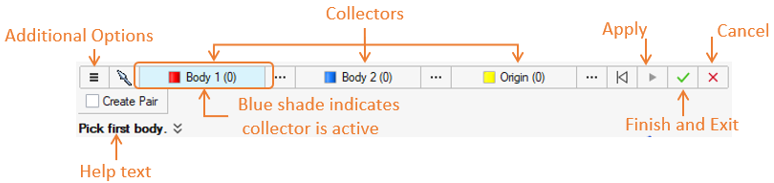
-
Select the CrankShaftNose body from the modeling window as the second body of the
joint.
Note: The CrankShaftNose body should now be highlighted in blue. The Origin collector is now highlighted, allowing you to pick an existing point or create a new point to define the location for the joint. Observe that in this point picking mode all the graphics are made translucent, thus providing a better view for picking a point.
Figure 14. Graphics Highlight in Context 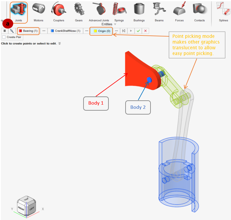
-
Create a point to define the joint’s origin.
- Hover near the center of the hole in the Bearing (the cylindrical surface) where it overlaps with the CrankShaftNose so that a red cross is displayed with the surface highlighted in white. Adjust the view as needed by rotating (middle mouse button) and zooming (scroll).
- Click to create a new point here and use it to define the joint’s origin.
Figure 15. Choosing a Joint Origin using CAD Reference 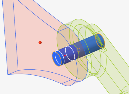
Note: Observe that a new point ‘Point 0’ has been added to the model (see Model Browser) and the Origin collector on the Guide Bar is now resolved to Point 0. Also, a microdialog with a Create button is now displayed since all the required references have been resolved.Figure 16. Joint Create/Edit Context 
Note: When a CAD geometry is available, geometrical references like straight/arc line center or end points, circle center, flat surface center, and so on can be used to create new points on the fly while resolving a collector as shown below.Figure 17. Using Geometrical References to Create Points 
-
Change the Joint type to Revolute from default
Ball.
Note: Observe that a new option Orient Axis (applicable to this joint type) appears on the Guide Bar.
Figure 18. Changing Joint Type using the microdialog 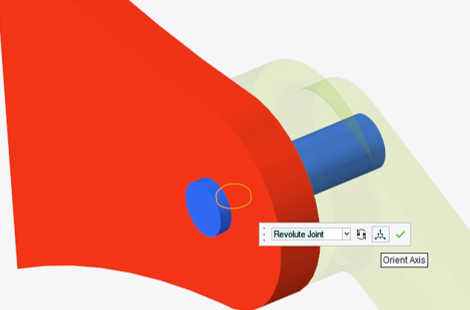
-
Click Orient Axis button
 on the microdialog
to enter the Orientation Context to orient the revolute joint
axis.
A vector tool appears that can be used to define the orientation of the revolute joint.
on the microdialog
to enter the Orientation Context to orient the revolute joint
axis.
A vector tool appears that can be used to define the orientation of the revolute joint.Figure 19. Vector Tool Available in the Orientation Context 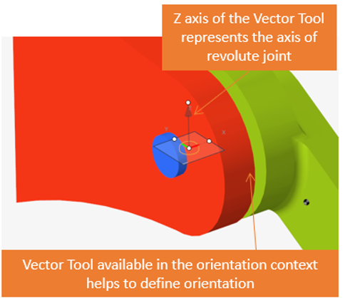
-
Drag around to find Global X axis direction.
Note: As the handle is dragged around, notice that it highlights points/vectors while hovering over CAD geometry as well as Global Axes while hovering in the empty space.
Figure 20. Global Axes Available for Joint’s Orientation 
-
Move closer to Global X label and notice that it gets highlighted with
an underline (Global X). Release the mouse to select it.
Tip: When selecting Global axes, release the mouse outside of any CAD geometry.
The Z axis of joint should now be aligned along the Global X direction.
Use the right-click Exit Context button
to exit the orientation and return to
the Joint context. -
Click the Finish Editing check mark button
on the Joint’s Microdialog to complete
defining the current joint.
Note: At this stage, the current joint edition is complete and the context enters the create joint state.
-
Go to the Model Ribbon tab and click on the
Joints icon under the
Entities group.
-
Create a revolute joint with CrankPin as Body 1,
PistonRod as Body 2, and the inner surface center of
Crank Boss as Origin of the joint. Choose
Global X as orientation direction for the
joint.
Figure 21. Revolute Joint between CrankPin and PistonRod 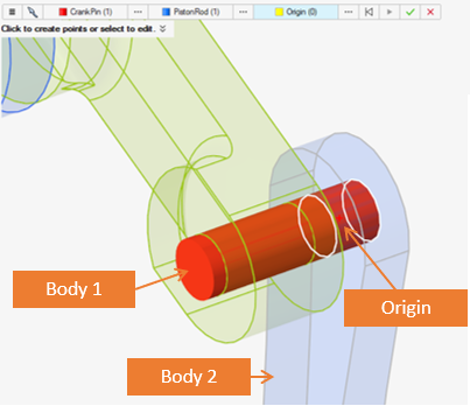
Note: Follow the same procedure for orientation as in the previous joint. -
Create another revolute joint with PistonRod as Body 1,
PistonPin as Body 2, and the surface center of the
PistonRod hole as Origin of the joint.
Figure 22. Revolute Joint between PistonRod and PistonPin 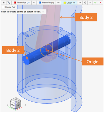
-
For orientation, change the pick method
 to Point. Use the edge center point of
Pistonrod hole as shown below. A new point Point
3 is created and the joint oriented using the Point
method.
to Point. Use the edge center point of
Pistonrod hole as shown below. A new point Point
3 is created and the joint oriented using the Point
method.
Figure 23. Revolute Joint between PistonRod and Piston 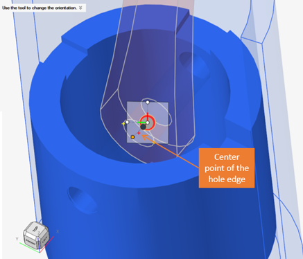
-
For orientation, change the pick method
-
Create a cylindrical joint with Piston as Body 1, Cylinder as Body 2, and the
outer surface center of the Piston as Origin of the joint. Choose Global Z as
orientation direction for the joint.
Figure 24. Cylindrical Joint between Piston and Cylinder 
Figure 25. Orientation Axis for the Cylindrical Joint 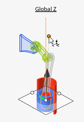
-
Exit the Joint context by using the Cancel button
 on the guide bar.
-
Save
 the model.
-
Fit the model to screen by clicking the Fit icon on the
View Controls toolbar.
Tip: Keyboard shortcut "F" can also be used to fit the model to screen.
Solve the Model
In this step, you will learn how to solve a model.
-
Run a transient analysis for 1 second.
-
From the Ribbon Bar, select Analyze and click on the
Quick Start/Stop Motion Analysis button from the
Solution group.
Figure 26. Perform a Quick Run 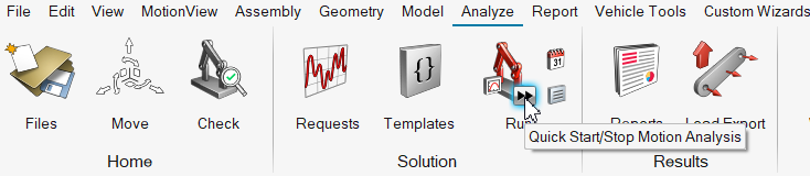
Note: MotionView performs a model check and then submits a run to MotionSolve. The motion of the model can be viewed in the MotionView window as the solution progresses. There are no forces defined in the model, still the parts move as they fall under default gravity.The Run Status dialog opens showing the status of the current run in progress.Note: Once the run is finished, a blue check mark appears near the Run icon in the ribbon indicating that run has been completed successfully and a result is available with the model. After the run, the mode is set automatically into Results Review Context indicated by the blue highlight on the Run icon.Figure 27. Review Run Results Context 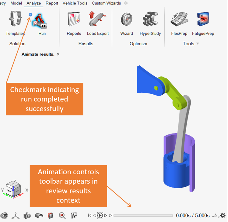
Review the Results
In this step, you will learn how to post-process your model results.
-
Use the Play/Pause button or drag the slider to review a
specific animation time frame.
Figure 28. Animation Controls 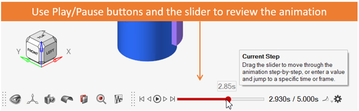
Note: Animated post-processing features in the MotionView client are limited. -
Create a plot.
- Click on the Plot button available on the Run status dialog (or right-click on the run entry and select “Plot Results on HyperGraph” from the context menu).
A new page with HyperGraph client is added to the session and Create Curves by File dialog appears. The MotionSolve result file (*.mrf) is pre-selected. -
Plot a curve that represents displacement of a Piston along the Cylinder.
- Select Body from the list of Types.
- Select the Part/76000000 PistonHead from the list of Requests.
- Select Z from the list of Components.
- Click Plot and then Cancel.
Figure 29. Plot a Curve in HyperGraph 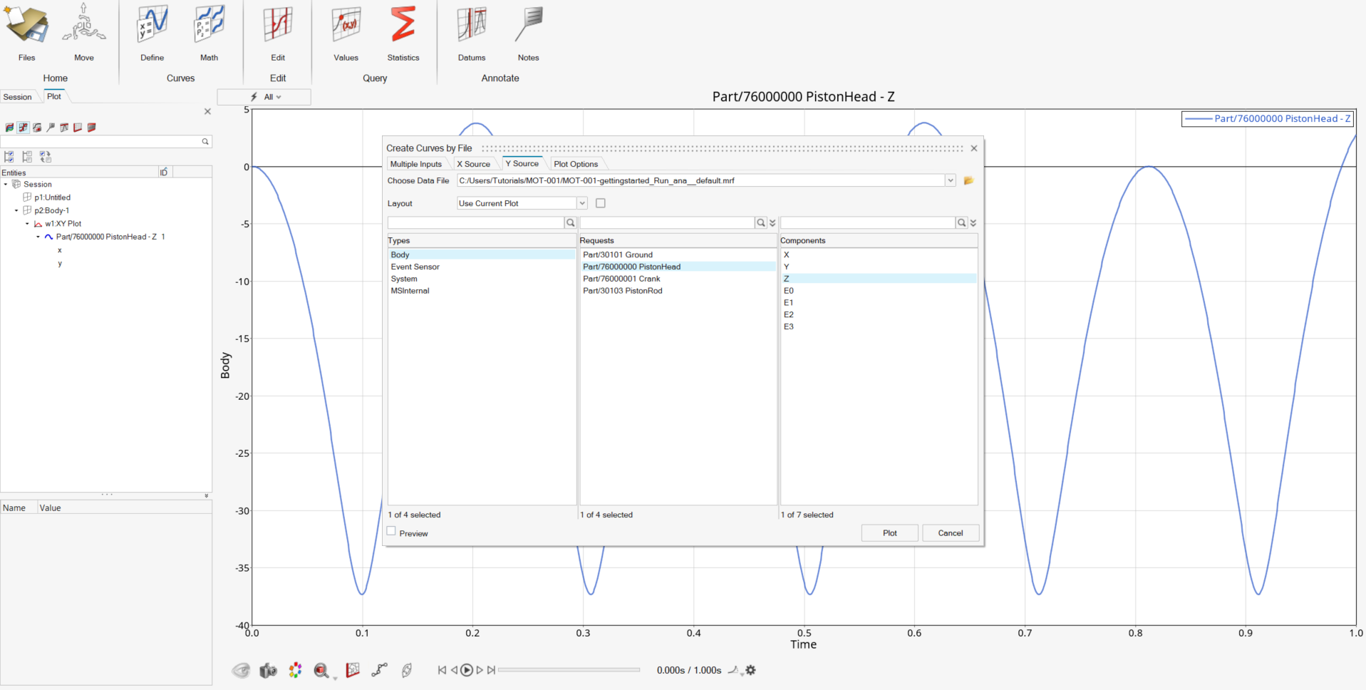
-
Navigate to the first page using the page navigation icons in the top right
corner of the application
 .
.
-
From the Menu Bar, click .
Figure 30. Saving a Session 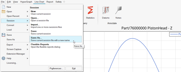
- Select the working directory and save the session file as MV_Getting_Started.mvw.