Tutorial Level: Advanced In this tutorial, you will learn how to setup a model in MotionView that will be coupled with AcuSolve through HyperMesh CFD.
Through this co-simulation interface, you can now solve multi-physics problems that
involve complex rigid body movement, coupled with fluid flow, that generates
pressure forces on the rigid bodies. This capability lets you enhance the fidelity
of your multibody system, letting you generate more realistic results.
In this scenario, MotionSolve computes the displacements
and rotations for the rigid bodies, while AcuSolve
computes the forces and moments on those bodies. Both solvers exchange data with
each other while stepping forward in time via the TCP socket protocol. This means
that the two solvers can be located on different machines and on different platforms
and still communicate with one another. For example, the CFD simulation can run on
an HPC, while the MBS simulation can run locally on a laptop.
Tutorial Objectives
You will use the MotionSolve-AcuSolve co-simulation interface to couple the rigid body
dynamics of a check valve within a pipe with the flow field. The AcuSolve model has already been setup for you in HyperMesh CFD.
Before you begin, copy the file(s) used in this tutorial to your
working directory.
Note:MotionSolve – AcuSolve
co-simulation can also be set up and executed using Altair/SimLab. The steps to
set up the MotionView model is the same as described
in this tutorial. To learn about setting up the fluid model in SimLab, please refer to tutorial SL2331 Coupled Simulation of a Check Valve using AS +
MS.
Software Requirements
To successfully complete this tutorial, the following software must be installed.
Each software is installed through an installer package.
Software
Installer Package
MotionView
hwdesktop
HyperMesh CFD
hwdesktop
MotionSolve
hwsolvers
AcuSolve
hwCFDSolvers
Note: All the above software can be installed at once
using the AltairHyperWorks Products installer (hw). Please refer to
the Installation Guide on how to install AltairHyperWorks Products.
The co-simulation is supported for both Windows and Linux
platforms (64-bit). Cross platform co-simulation is also possible.
Simulation Environment
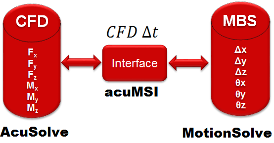
The co-simulation interface between MotionSolve and
AcuSolve consists of a “middleware” utility
executable, acuMSI.exe. This executable is responsible for:
Establishing a connection to both MotionSolve
and AcuSolve.
Communicating the displacements and rotations from MotionSolve to AcuSolve.
Communicating the forces and moments from AcuSolve to MotionSolve.
Managing runtime and licensing.
This is shown schematically below.Figure 1. Co-Simulation setup
Pipe with a Check Valve
A check valve is a mechanical device that permits fluid to flow in only one
direction. This is controlled by a shutter body. Fluid flowing in one direction
pushes the shutter body in one direction, thereby opening the valve. Fluid flowing
in the opposite direction pushes the shutter body in the other direction, which
causes the valve to shut and prevents flow reversal in the pipe. Check valves are
found in pumps, chemical and power plants, dump lines, irrigation sprinklers,
hydraulic jacks, for example.
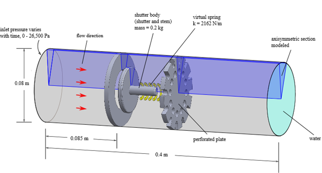
The geometry that is modeled in this tutorial is illustrated in the figure below. It
consists of:
A pipe with an inlet and outlet for the fluid flow.
A check valve assembly that consists of a shutter plate attached to a
stem.
A stop mounted on a perforated plate downstream of the shutter body.
The fluid flow in the pipe is assumed to be axisymmetric. This allows you to
model only a part of the check valve. In this example, a 30-degree section
of the geometry is modeled, as shown by the blue part in the figure below.
The advantage of doing this is a reduced simulation time while still
capturing an accurate solution.
Figure 2. Pipe with check valve model setup
The check valve assembly consists of a disc-like body mounted on a stem. When fluid
flows in the direction specified by the red arrows in the figure above, the fluid
forces the shutter body to translate in the same direction as the fluid. The motion
of the shutter body is also affected by a spring damper attached between the shutter
body and the perforated plate. Finally, 3D rigid body contact is modeled between the
shutter body and the stop to arrest the motion of the shutter body in the direction
of the flow.
For the MBS model, only 1/12 of the shutter body and the perforated plate are
modeled.
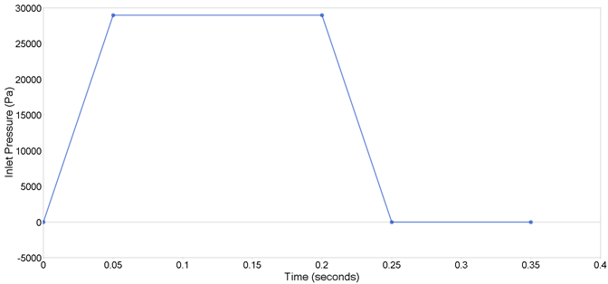
At the start of the simulation, the flow field is stationary. A pressure specified at
the inlet drives the flow, which varies over time as a piecewise linear function.
This is illustrated in the figure below. As this pressure rises, the flow
accelerates which in turn pushes the shutter body open and allows flow through the
pipe.Figure 3. Inlet pressure
This dynamics of this kind of model can be termed as being “tightly” coupled between
the two solvers. This means that the motion of the rigid bodies affects the fluid
flow field, which in turn affects the rigid body motion in a cyclical fashion.
The rest of this tutorial assumes that this model has been correctly setup in
HyperMesh CFD. Note that the model is designed to translate
the shutter body until it collides with the perforated plate. The MotionView model has been designed with a contact between
these two bodies that causes the shutter body to rebound appropriately. To allow the
rigid bodies to come into contact without the CFD finite element mesh fully
collapsing, the perforated plate in the fluid model has been offset by 0.002m in the
positive X direction.
Load the Model in MotionView
From the Start menu, select Altair <version> MotionView <version>.
If the HyperWorks Launcher is seen, click on
Create Session to start a MotionView session.
Click and open the model
Valve_model.mdl.
This model is prepared to run in MotionSolve
but requires modifications to run in co-simulation with AcuSolve. These steps are outlined below.
Once the
model is loaded into MotionView, the graphical
window displays the shutter body, perforated plate, joint and spring
entities, as well as a graphical representation of the spring damper as
shown in the figure below.Figure 4. The MotionSolve model of the pressure
check valve
The MotionSolve model consists of the following
components:
Component Name
Component Type
Description
Ground Body
Rigid Body
Ground Body
Shutter Body
Rigid Body
30-degree section of the shutter body.
Shutter Body Graphic
Graphic
The graphic that represents the shutter body. This
graphic is used for the contact force
calculations.
Perforated Plate Graphic
Graphic
The graphic represents the perforated plate belonging
to Ground Body. This graphic is used for the contact
force calculations.
Contact
3D Rigid-Rigid Contact Force
3D rigid-rigid contact force between the Shutter body
and the Ground Body (Perforated Plate).
Solver Units
Data Set
The units for this model (Newton, Meter, Kilogram and
Second).
Note: The units in the
MotionSolve and
AcuSolve models need
not match to run the co-simulation; however, the
units must match to overlay the results animations
in HyperView.
Gravity
Data Set
Gravity specified for this model. The gravity is
turned on and acts in the negative Y direction.
Spring
Graphic
The graphic that represents the spring modeled
between the shutter body and the perforated plate body.
This is only for visualization and does not affect the
co-simulation results.
Translation
Translational Joint
This translational joint allows motion of the shutter
body along the X axis.
Spring
Spring Damper
This is a simple spring damper mounted between the
shutter body and the Ground Body.
ContactOutput
Output
An output signal that measures the contact
force.
Displacement
Output
An output signal that measures the displacement
between the shutter body and the ground.
Velocity
Output
An output signal that measures the velocity of the
shutter body with respect to the ground.
Run the Model without Co-simulating with AcuSolve
To verify that the MotionView model is set up correctly,
run the model in MotionSolve and verify that there are
no warning/error messages from MotionSolve.
From the Analyze ribbon, click Analysis
settings, , to display the
Run Motion Analysis dialog.
Provide a Run nameValve_Model_no_cosim.
Specify an Output directory.
Click Run
Review the log by clicking View Log on the
Run Status dialog. Verify that the MotionSolve run is complete and there are no errors.
Close the Run Status dialog.
Notice that there is no motion in any of the parts. This
is because the actuation for this model comes from AcuSolve,
which is not yet enabled.
Open the Fluid Model
In this step, you will open the fluid model prepared in HyperMesh CFD.
From the Start menu, select Altair <version> HyperMesh CFD <version>.
Open the model Check_Valve_Coupled.hm from the working
directory.
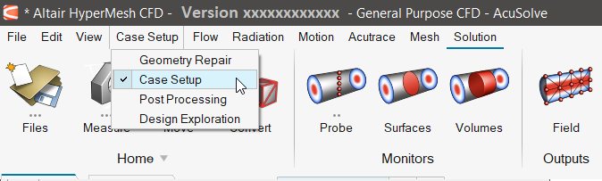
Switch to Case Setup as shown in the image below:
Figure 5. Case Setup Ribbon
Note: This model has already been set up for
co-simulation. To learn about building a HyperMesh CFD
model for co-simulation with MotionSolve, please
refer to the tutorial ACUT-5021.
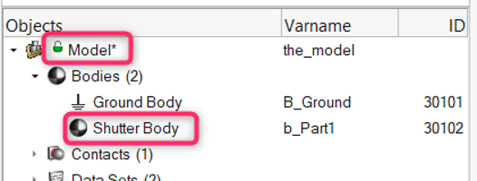
For a successful coupling, the names of the interacting bodies need to match
between MotionSolve and AcuSolve.
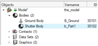
In the MotionViewModel Browser note the hierarchy and label of the
Shutter body that will be interacting with the fluid domain. That would
be Model-Shutter Body, which is the full label of
the body that would be identified by MotionSolve during the simulation.
Figure 6. Interacting body's label
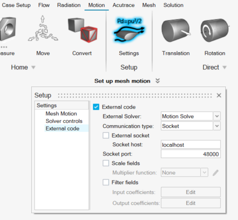
In HyperMesh CFD, go to the
Motion ribbon. Click on the
Settings icon under Setup group to display
the Setup dialog.
Make sure the External Solver selected is Motion
Solve. Retain other settings for socket as
default.
Figure 7.
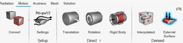
Click on the External Surfaces icon under the
Derived group to bring up the External Code surfaces tool.
Figure 8.
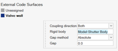
The Valve surface is already defined for this model. Right-click on
Valve-Wall from the list of External Code
Surfaces on the left of the screen. This is the fluid surface that would
interact with the Shutter Body in the MotionSolve model. Confirm that the text for the
Rigid body reads Model-Shutter Body as noted in
MotionView previously.
Figure 9.
Exit the tool .
Set Up Interaction
To couple with AcuSolve, you need to specify one or more
"wet" bodies. A "wet" body is a body in the MotionSolve
model which interacts with the fluid flow and thus has forces and moments acting on
it. Such a body can translate or rotate due to the actuating fluid force/moment as
computed by AcuSolve as well as due to any actuating
forces/moments in the MotionSolve model. In this
example, you will define a single "wet" body – the Shutter body that translates
along the X axis due to fluid impinging on it.
To specify a body as "wet" in MotionView:
From the Project Browser, select the body
Shutter Body.
Figure 10. Selecting the Shutter BodyThe properties are displayed in the Entity Editor.
Note: If the Entity Editor
is not visible, turn it on from the View
menu.
From the Properties section, select Fluid interaction with AcuSolve
Figure 11. Enabling Fluid Interaction with AcuSolve
Run the Co-simulation
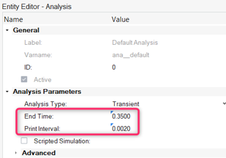
Verify that the end times for both models are set to the same values. For this
tutorial, the end times for both the AcuSolve and
MotionSolve runs are set to 0.35s. Also, the
print_interval for the MotionSolve model needs to match the step size for the
AcuSolve model. It is set to 0.002s.
To verify the motion model, select Default
Analysis from Model Browser in
MotionView.
From Entity Editor, view the
Analysis Parameters.
Figure 12. Analysis Parameters
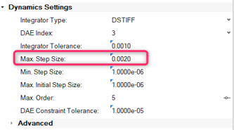
Verify that the MotionSolveMax Step Size, h_max, matches
the Print Interval (0.002s in this case).
Figure 13. MotionSolve Maximum Step
Size
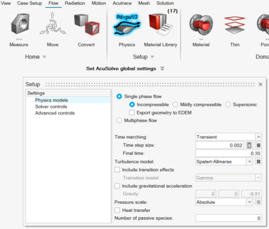
In HyperMesh CFD, go to the Flow ribbon and click on
Physics under the Setup group.
Set the Time step size to
0.002 and Final time
to 0.35.
Figure 14.
There are two methods to execute the MotionSolve
solver.
Live through MotionView.
In this mode, the simulation progress with the
motion model can be seen in MotionView
through live animation of the model. This method is useful for a
model with medium complexity and size, where run times are not
large.
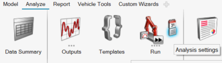
From the Analyze ribbon, click on the
Analysis settings icon.Figure 15.
In the Run Motion Analysis dialog, provide a Run
name.
Provide an Output directory.
Click Run.
The Run Status dialog appears and MotionSolve is initiated and will wait
for the coupling.
Note: Based on firewall settings, a pop-up
window could appear asking for permissions to start the coupling
exe.
Go to Step 6 to start the run in HyperMesh CFD.
Offline through Altair Compute console.
This
method is useful for large CFD models that needs to solve on a
cluster with higher computing power.
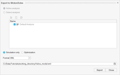
Export the solver deck to your working directory, click
File > Export > Solver Deck.Figure 16. Exporting the model to .xml
Select Simulation Only and Format as
XML.
Provide a file name and click
Export.
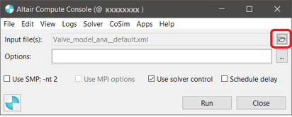
From the Start menu, select All Apps > Altair <version> > Compute
Console and select MotionSolve as the
solver. Locate the model you just exported by clicking on the
file open icon.Figure 17. Select the exported model from disk
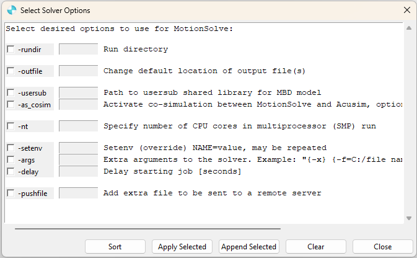
Click the ellipsis button next to the
Options field to open the Select
Solver Options dialog.Figure 18. Selecting the co-simulation flag
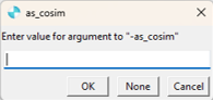
Activate the –as_cosim option. When you
activate this option, the following dialog is displayed and you
are prompted for additional options:Figure 19. Specifying options for the co-simulation
You may specify the following options here:
acuMSI Options
-aport <integer>
Specifies the communication port number for
communication between AcuSolve and acuMSI. The
default is 48000.
Note: If
you need to change the default port for
communication between AcuSolve and acuMSI, in
addition to changing this argument, you also have
to specify the changed port number in the AcuSolve input file.
-mport <integer>
Specifies the communication port number for
communication between MotionSolve and acuMSI. The
default is 94043.
Note: If you need to change
the default port for communication between
MotionSolve and
acuMSI, in addition to changing this argument, you
also have to specify the changed port number in an
environment variable MS_AS_PORT. MotionSolve checks for this
environment variable at the start of the
simulation and changes its listening port
accordingly.
-mi <integer>
Specifies the maximum number of iterations per
time step between the two solvers. The default is
0.
-v <integer>
Specifies the verbosity level of the output file
from acuMSI. The default is set to 0 (verbosity
OFF).
To retain the default options, click
None.
Click Apply Selected and
Close.
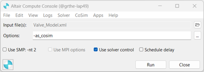
You are now set up to start the co-simulation on the MotionSolve side. Click
Run.Figure 20. Run the MotionSolve
model
This launches MotionSolve as well as
the acuMSI executable. The MotionSolve
run is paused at the first time step – it is now in waiting mode and
the co-simulation will start as soon as AcuSolve is run. Figure 21. The MotionSolve simulation is
waiting for a connection to AcuSolve
Run the AcuSolve Executable for
Co-simulation
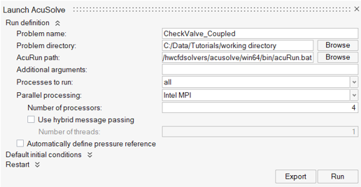
From the Solution Ribbon tab in HyperMesh CFD, click the Run icon to invoke the Launch AcuSolve dialog.
Set Problem name as
Check_Valve_Coupled.
Make sure that Problem directory is set to your current
working directory. Use the Browse button to search for
your working directory folder.
Set AcuRun path as
.../~altair_install/hwcfdsolvers/acusolve/win64/bin/acuRun.bat,
found in the installation.
Click Run to initiate the simulation in AcuSolve.
Figure 22. Launching AcuSolve for the
co-simulation
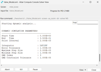
As the solution starts, the Run Status dialog is
opened, where you can watch the simulation’s progress. HyperMesh CFD generates the input files and launches AcuSolve.
Soon, AcuSolve and MotionSolve should begin to communicate with one
another. You should be able to see relevant time stepping information in
both solver windows. For example, you should see something like the
following in the MotionSolve window at the
beginning of the
co-simulation:
INFO: [AS-COSIM] Connected to AcuMsi on port 94043
INFO: [AS-COSIM] License checked out.
…
Time=2.000E-06; Order=1; H=2.000E-06 [Max Phi=1.314E-16]
Time=3.600E-02; Order=2; H=2.000E-03 [Max Phi=1.653E-08]
…
The co-simulation should take roughly 15 minutes to complete on a laptop
(Intel i7. 2.8GHz).
Note that there is no order dependency on launching the co-simulation –
either MotionSolve or AcuSolve can be launched first.
Post-process the Results from the Co-simulation
HyperView and HyperGraph can
be used to post-process the co-simulation results within a session.
The animation H3D generated by the MotionSolve
part of the co-simulation contains only the results from MotionSolve. Similarly, the result files from AcuSolve only contain the results for the AcuSolve model. To animate the results from the
co-simulation, follow these steps:
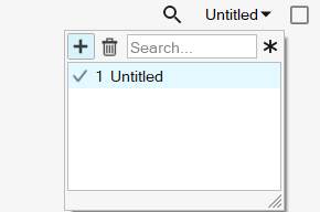
Add a page to the MotionView session by clicking on
the session page list drop-down on the toolbar at the top right corner and click
+.
Figure 23.
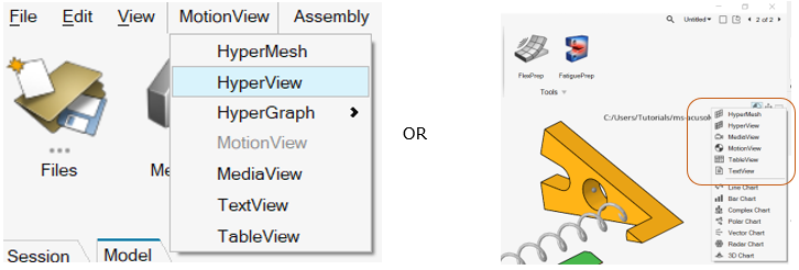
Change the client of the newly added page to HyperView either from the menu bar or the top right of the modeling window.
Figure 24.
Load the animation H3D generated by MotionSolve in
HyperView.
Click on the Open icon to display the Load model and results
panel.
Note: If the panel is not visible, turn on the
panel from the View menu.
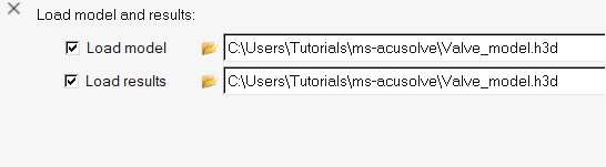
Click the file open button, , next to Load model and navigate to the results
directory (the same directory where the .xml file
is located).
Select the .h3d file and click
Open.
Click Apply.
Figure 25. Loading MotionSolve H3D in
HyperView
Click the Play icon on the Animation toolbar to animate the motion
result.
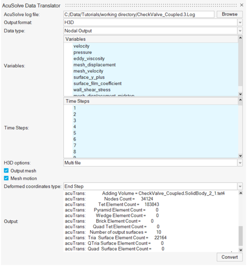
To load the AcuSolve results, they must first be
converted to the .h3d format. This can be accomplished by
using the Convert tool in HyperMesh CFD.
In the Solution Ribbon, click on the Convert icon .
Use the Browse button to load the solver’s
.Log file as the AcuSolve log file parameter.
Select H3D as the Output Format from the drop-down
menu.
Select all variables in the Variables section, by
clicking on a variable and using ctrl + A on
Windows.
Similarly, select all Time Steps.
Figure 26. Generate AcuSolve H3D file
Click Convert. This creates a single
.h3d file containing all the time steps available for
the simulation.
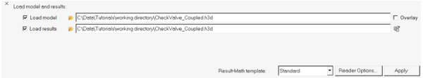
Using HyperView, overlay the newly-created H3D over
the MotionSolve result H3D in HyperView. This is accomplished by repeating Step 1
described above and activating Overlay when selecting the
AcuSolve result H3D.
Figure 27. Overlaying AcuSolve H3D over the MotionSolve H3D in HyperView
Click Apply.
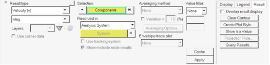
Once loaded, the modeling window contains both
results and can be animated as before. To visualize the information
contained within the AcuSolve results, a Contour
plot may be used.
Click on the Contour button to display the panel.
Set the options as shown in the figure below and click
Apply.
Figure 28. Visualizing flow velocity using Contour
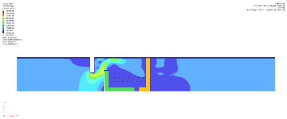
This creates a contour plot of the velocity magnitude overlaid with the
results from MotionSolve in one window.Figure 29. Velocity magnitude plot overlaid with the MotionSolve results in HyperView
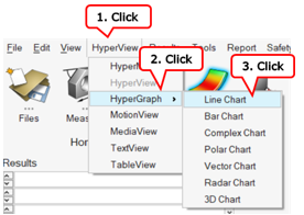
Plotting the MotionSolve Results in HyperGraph
You can also interpret the results with a
two-dimensional plot using HyperGraph. Use the
multi-window layout, allowing both HyperView and
HyperGraph to be open at the same
time.
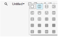
From the top right corner, click the Set Page Layout
button and split the page into two vertical pages.
Figure 30. Splitting the page into two vertical pages
This automatically adjusts the modeling window to
accommodate two pages, defaulting to two instances of HyperView.
Click anywhere in the page on the right and switch to HyperGraph by clicking the Client
Selector to select HyperGraph from
the drop-down list (as shown in the figure below).
Figure 31. Open HyperGraph
Click the Open Plot button to load the
.plt file from the same results directory.
Once the .plt file is loaded into HyperGraph, the two outputs are available for
plotting.
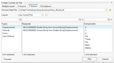
In the Y Source tab, perform the following
selections:
Under Types, select Displacement.
Under Requests, select REQ/70000002 Shutter Body from
Ground Body(Displacement).
Under Component, select X.
Click Plot.
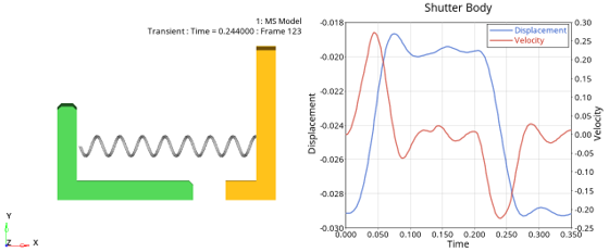
HyperGraph can be used to create additional
traces on the same plot to generate the following plots.Figure 32. Select the signals for plotting Figure 33. Visualizing Shutter body results
 and open the model
Valve_model.mdl.
This model is prepared to run in MotionSolve but requires modifications to run in co-simulation with AcuSolve. These steps are outlined below.Once the model is loaded into MotionView, the graphical window displays the shutter body, perforated plate, joint and spring entities, as well as a graphical representation of the spring damper as shown in the figure below.
and open the model
Valve_model.mdl.
This model is prepared to run in MotionSolve but requires modifications to run in co-simulation with AcuSolve. These steps are outlined below.Once the model is loaded into MotionView, the graphical window displays the shutter body, perforated plate, joint and spring entities, as well as a graphical representation of the spring damper as shown in the figure below.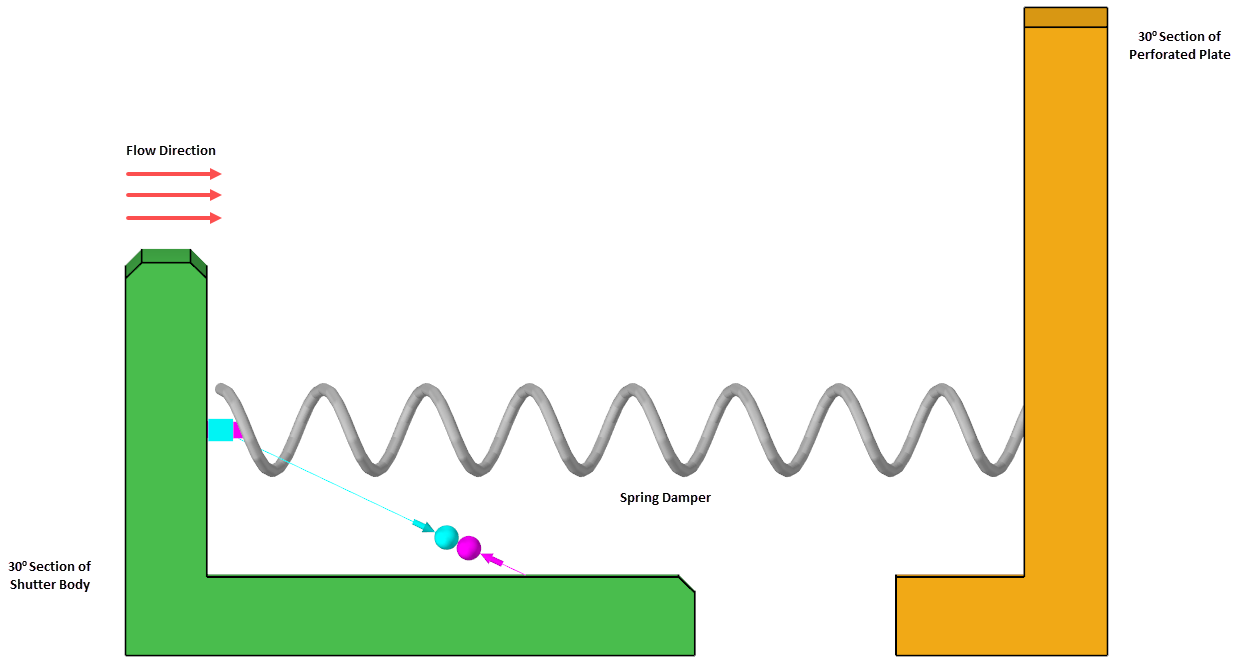
 , to display the
Run Motion Analysis dialog.
, to display the
Run Motion Analysis dialog.
 .
.
 Note: If the Entity Editor is not visible, turn it on from the View menu.
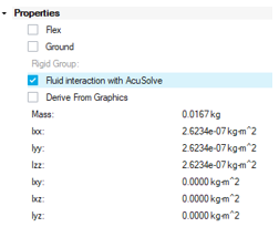
 to invoke the Launch AcuSolve dialog.
 , next to Load model and navigate to the results
directory (the same directory where the .xml file
is located).
, next to Load model and navigate to the results
directory (the same directory where the .xml file
is located).
 on the Animation toolbar to animate the motion
result.
on the Animation toolbar to animate the motion
result.
 .
.