Full Car Model with Dual Motor Electric Powertrain
In this tutorial, you will learn how to use MotionView to build a full vehicle model with a Dual Motor Electric Powertrain, adjust its motor characteristics, and simulate over a WLTP cycle road event.
The Worldwide harmonized Light vehicle Test Procedure (WLTP) is a global standard used to measure fuel consumption and CO2 emissions from passenger cars and vans, as well as their pollutant emissions. This procedure establishes a distinct speed profile, along with various testing conditions, to accurately mirror real-world driving behaviors across a wide spectrum of driving scenarios.
The vehicle’s powertrain architecture comprises one motor per axle, each paired with an inverter, a gearbox, and a differential. A battery pack is also available to provide sufficient power to the motors. The motors, inverters, battery pack, and Vehicle Control Unit (VCU) are all represented in an FMU file created using Altair Twin Activate. The VCU is responsible for managing various aspects, including vehicle regenerative braking, throttle response, and the distribution of torque between the front and rear axles of the vehicle. Finally, the motors’ information is provided by external files that contain their torque curves and efficiency maps.
Model Overview
- Open a new MotionView session.
-
From File, click and load the Vehicle Tools
extension.
Figure 1. Load Vehicle Tools 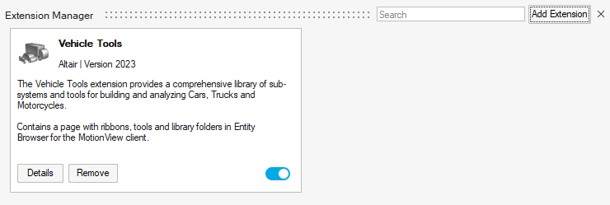
-
From the Vehicle Tools ribbon, click on the Assembly
icon to open the Assembly Wizard.
Figure 2. 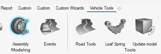
-
Select Full vehicle with driver from the wizard and
click Next.
Figure 3. Select Type of Model 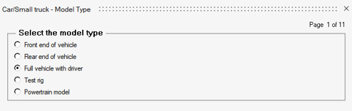
-
Select the Four Wheel Drive option for driveline
configuration and click on Next.
Figure 4. Select Driveline Configuration 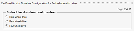
-
In Primary systems page, select Dual Motor Electric Powertrain
(FMU) under powertrain.
Figure 5. Select Type of Powertrain 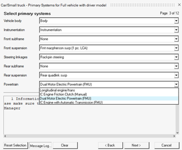
- Complete the model creation with the default selections by clicking on Next.
-
Review the model.
For more information on the Dual Motor Electric powertrain, please refer to the Dual Motor Electric Powertrain topic.
Figure 6. Dual Motor Electric Vehicle Model 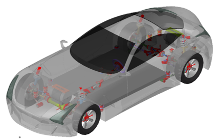
Access Motor Information
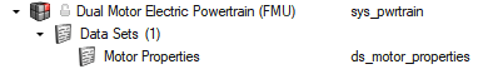
- In the Model Browser, expand the Dual Motor Electric Powertrain (FMU) system.
-
Locate the Motor Properties dataset menu under
Data Sets. In Entity Editor,
there are two files:
- Motor properties file - front
- Motor properties file - rear
Figure 8. Motor Properties File 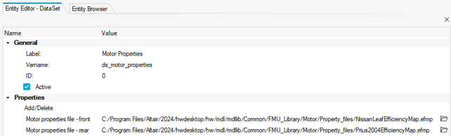
Both contain information regarding each motor’s efficiency and maximum torque. This data is organized in teimorbit format files and is derived from the FMU to contribute to motor control.
The default files consist of two motors with different specifications. Specifically, the first section of the file contains data related to the efficiency map of the motors. Motor’s torque limits data is included in the file’s second section.
Figure 9. Motor Properties .efmp File 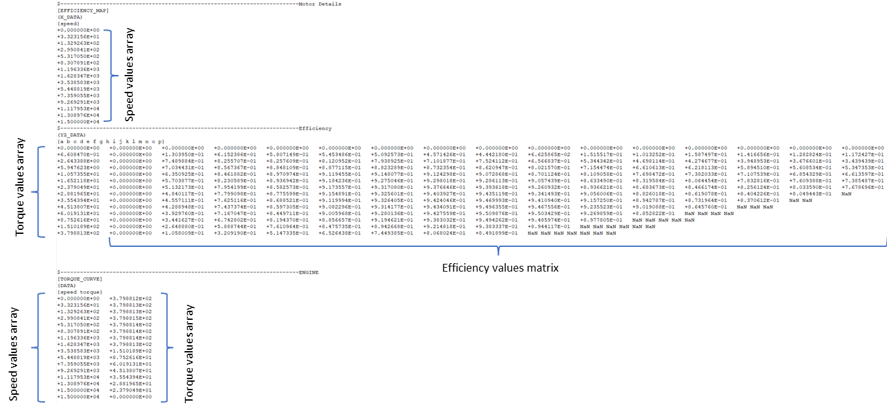
-
To replace the front motor with a new one, click on the
open icon
 and select the ‘Front_Motor.efmp’ file from the tutorial
folder. Repeat the process for ‘Rear_Motor.efmp’ to also
change the rear motor.
and select the ‘Front_Motor.efmp’ file from the tutorial
folder. Repeat the process for ‘Rear_Motor.efmp’ to also
change the rear motor.
Figure 10. Selected Motor Property Files 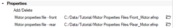
The front motor has a power output of 64.5 kW and a rated torque of 382 Nm, while the rear motor has a power output of 97 kW and a rated torque of 219 Nm.
Instead of using new files, you can also try to modify the existing ones by saving them in a directory separate from the system’s installation.
Select a Torque Distribution Strategy
-
Click on the FMU Dual Motor and select
Edit in Entity Editor.
Figure 11. FMU Properties Section in Entity Editor 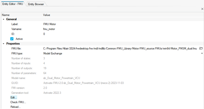
-
Within the FMU, the VCU defines a torque distribution strategy, with respect to
system’s efficiency optimization. Currently, there are four options available:
‘Evenly Distributed’, ‘Single Axle’, ‘Switch after Threshold’ and ‘Optimal
Torque Ratio’.
- Evenly Distributed (ED): The torque distribution is evenly split between the front and rear axles, constituting a 50-50 balance. Input 1 as ‘vcu_type’ parameter value to select this control strategy.
- Single Axle (SA): all of the torque is directed to the rear axle, representing a 100% rear axle torque distribution. Input 2 in ‘vcu_type’ parameter to select.
- Switch after Threshold (ST): the power losses are calculated and the VCU selects between SA and ED, with respect to power loss reduction. Input 3 in ‘vcu_type’ parameter to select.
- Optimal Torque Ratio (OTR): an optimal 3D torque map is formed offline, that establishes the optimum torque distribution in the range 0-100%, for all possible speed- torque demand scenarios. During the simulation, the right torque distribution is decided using it as a Look-up Table. Input 4 in ‘vcu_type’ parameter to select.
-
Navigate to parameters section, locate parameter
vcu_type and pick value 3.
This way, the torque distribution strategy ‘Switch after
Threshold’ is selected.
Figure 12. Torque Distribution Method Selection 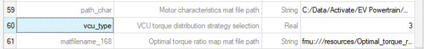
Modify FMU Parameters (Optional)
- Throttle response: the powertrain’s throttle response primarily depends on two key parameters: ‘traction_gamma’ and ‘traction_max’. Increasing ‘traction_gamma’ leads to a logarithmic increase in throttle’s responsiveness. ‘traction_max’ is used to linearly adjust the throttle pedal’s responsiveness.
- Regenerative braking: you can determine regenerative braking amount as a percentage of motors’ maximum torque capabilities, by modifying the ‘pedal_0_vx’ and ‘pedal_0_regen_percent’ parameters. The former represents a vector of velocities, while the latter is a vector that contains the corresponding regenerative braking percentages. This combination forms a map defining the regenerative percentage based on the cruising velocity. Vehicle’s coasting boundaries ‘pcl’ and pcu’ are defined by the parameters ‘coastm’, ‘coastphi’, ‘coastch’ and vehicle’s maximum velocity ‘max vehicle speed’. Finally, ‘regenpsi’ is employed to establish the correlation between throttle and output torque.
- Inverter/Converter: ‘inverter_efficiency’ and ‘converter_efficiency’ parameters are utilized to specify the efficiencies for considering power losses.
-
Battery Pack: ‘battery_charging_losses’ and
‘battery_discharging_losses’ parameters are used to model power losses during
charging or discharging. Battery’s capacity is determined by the following
parameters:
- nominal_voltage_cell: battery cell’s nominal voltage
- Capacity_cell: battery cell’s capacity
- num_modules_pack_parallel: Number of module packs in parallel
- num_cells_per_module_parallel: Number of cells per module in parallel
- num_cells_per_module_series: Number of cell rows per module
- num_modules_pack_series: Number of module packs rows
Initially designed as a 400V battery package, the most direct way to change its capacity is by adjusting the number of ‘num_modules_pack_parallel’ and ‘num_cells_per_module_parallel’.
Set an Altair Driving Event
-
You will now specify a driving event to simulate over a part of the urban WLTP
cycle. From the Model Ribbon, in the Splines toolset, select
Spline2D to add a curve.
Figure 13. Splines Toolset 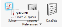
Note: From the menu bar select View > Panels, to enable Spline editing through panels. -
Specify Label and Variable name
as
WLTP velocity curveandcrv_wltp_velocity_curverespectively.Figure 14. Define Curve’s Label and Variable Name 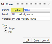
-
In panels sections, select the WLTP.csv file from the
tutorial directory as follows:
x y File WLTP.csv WLTP.csv Type Unknown Unknown Request Block 1 Block 1 Component T V Figure 15. Curve's Properties Panel 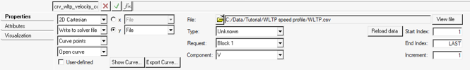
-
Check the curve shape to make sure the correct values are selected, by clicking
on Show Curve.
Figure 16. WLTP Cycle 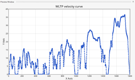
-
From the Entity Browser, navigate to and double-click on the Road Course
event.
Figure 17. Choose an Event 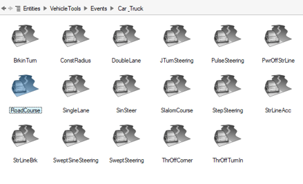
-
In the Entity Editor, label the Event as ‘
WLTP
                        cycle
’ with Varname ‘wltp’. -
From the Parameters section, go to Velocity
Profile and pick:
- ‘m/s’ in the Units drop-down menu
- ‘Curve’ in the Type drop-down menu.
-
Under the Curve settings section, select WLTP velocity
curve as Velocity Curve by
double-clicking on the Advanced Selector
 and set the end time at 60s.
Figure 18. RoadCourse Event Entity Editor 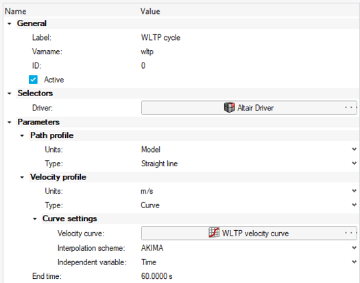
-
Then, from the Road settings section, select Road File
as Road selection and
‘2D_Flat_07mu.rdf’ as Road property
file. This file specifies a road with 0.7 friction
coefficient.
Figure 19. Adding a Road File 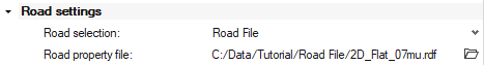
Simulation and Post-Processing
-
Under the Vehicle Tools ribbon, go to Run and open the
Analysis settings dialog.
Figure 20. Open Run Motion Analysis Settings Dialog 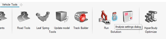
- Create a run folder as Output directory to write the results and pick a Run name of your preference.
- Click on Global Simulation settings…, select General under Analysis Settings and choose XML, as the Offline run solver file type.
-
Verify that the Run Offline check box and click the
Run button.
Figure 21. Run Motion Analysis Dialog Parameters 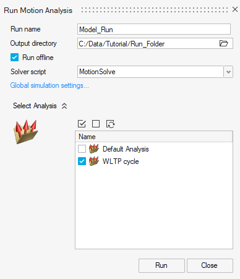
- The model initialization process begins, the ‘Run template’ executes the ‘MotorProperties.py’ file, which is responsible for generating the .mat files that contain the motors’ information. These files will appear in the run folder and are specific to the simulation’s run name.
-
After the simulation finishes, open a new HyperView window to visualize the
results.
-
Click on the Open Model button, load the
.h3d file in the panel, and click
Apply.
Figure 22. Open Model 
Figure 23. Load .h3d File 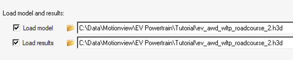
-
Click on the Open Model button, load the
.h3d file in the panel, and click
Apply.
-
From the Animation toolbar, click the
 (Start/Pause Animation) button to animate the
model.
(Start/Pause Animation) button to animate the
model.
- Add a new HyperWorks page.
-
Select the HyperGraph> Line
Chart application.
Figure 24. Switch to HyperGraph to Plot the Results 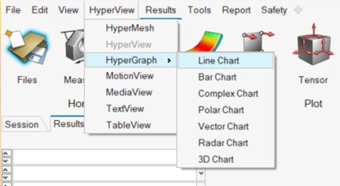
- Click on Open plot and load the .plt file from the MotionSolve run.
-
Select the 6-grid layout from the top-right corner of the menu bar.
Figure 25. Select a Suitable Page Layout 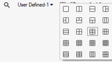
-
Select the following results file outputs from User
Defined type:
- Vehicle CG Velocities
- Battery Management → SOC
- Motor Management Rear → Torque Bias
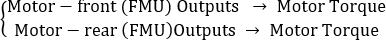
Figure 26. Plotting Outputs in HyperGraph 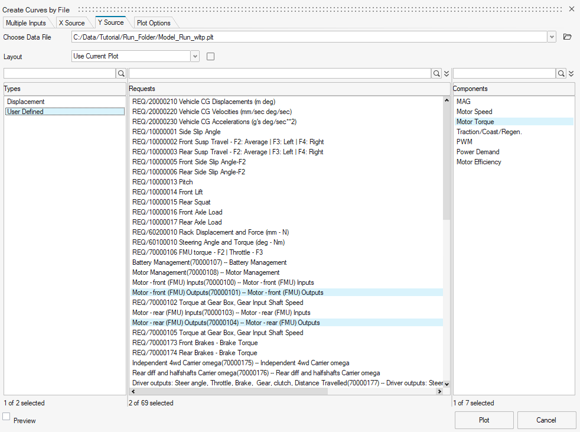
Figure 27. Simulation Results 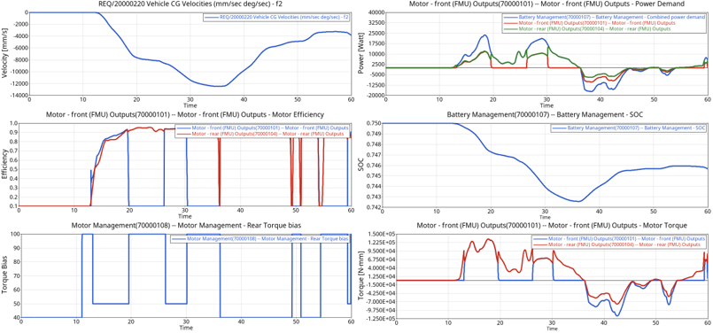
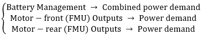
These results contain important information for monitoring vehicle’s overall efficiency, power consumption and torque distribution.- Top-Right Plot: This plot displays the power demand inputs from each motor's inverter to the battery pack, along with the combined power from both motors. Positive values indicate discharging (tractive) regions, while negative values represent charging (regenerative) regions.
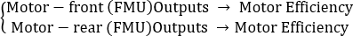
- Middle-Left Plot: In this plot, you can observe the efficiency of the motors as they vary over time.
- Middle-Right Plot: This plot illustrates the state-of-charge of the battery. A decrease in the state-of-charge is a result of battery discharge, while an increase is due to charging from regenerative braking.
- Bottom-Left Plot: Here, you can find the torque distribution ratio, which is determined by the 'Switch after Threshold' method. This method dynamically switches between values 0.5 (ED) and 1 (SA), depending on power losses and 0.4 during regenerative braking. The selection of a 0.5 ratio at this point significantly minimizes power losses, when compared to the 1(SA) setting.
- Bottom-Right Plot: This plot displays the torque outputs of both motors. Positive values indicate the tractive region, while negative values represent the regenerative braking region.
Optionally, you can repeat this process for different torque distribution strategies by selecting a different ‘vcu_type’ in the third step of the tutorial. For example, choosing the ‘Optimal Torque Ratio’ method would result in a different torque bias diagram, utilizing all possible torque ratios in the range of ‘0-1’. This, in turn, leads to different power consumption for the same speed profile.
Use FluxMotor to export motor property files (Optional)
-
Start FluxMotor and click on Motor
Catalog.
Figure 28. 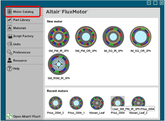
-
In motor catalog, choose Automotive Transport and
double-click on the Nissan Leaf icon.
Figure 29. 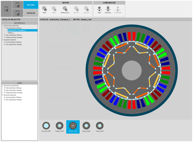
-
Specify the Motor Name as
Nissan_Leaf_1, keep Catalog Name asUser_SM_PM_IR_3Phand click the Check button to open the Motor Factory.Figure 30. 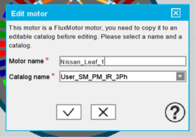
-
Click on TEST and then on PERFORMANCE MAPPING
– Sine Wave to specify the type of analysis.
Figure 31. 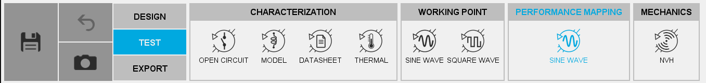
-
The analysis inputs are displayed in the SINE WAVE
dialog.
Figure 32. 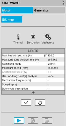
-
Click on Thermal menu and enter the following thermal
settings:
- Winding straight part temperature: 150 ℃
- C.S. end winding temperature: 150 ℃
- O.C.S. end winding temperature: 150 ℃
- Magnet temperature Tmag: 100 ℃
Then, click on the Check button to apply settings.Figure 33. 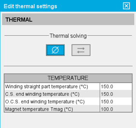
-
Click on the Start icon to launch the analysis.
Figure 34. 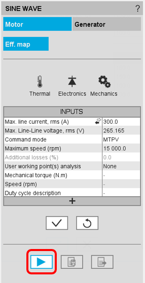
-
After the FluxMotor analysis is finished, you can
review the results of motor’s performance and click on Export
results icon to save them.
Figure 35. 
-
In the Export results dialog, enter the Export name as
NissanLeafEfficiencyMapand set the Destination folder as your <working directory>. -
Make sure you have selected all the check boxes as shown below and click on the
Check button:
Figure 36. 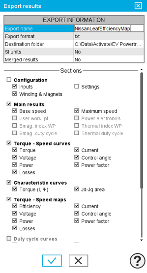
FluxMotor exports 27 .txt files containing the motor’s characteristics. From these, two files will be used to create the efficient map file used in the Dual Motor Electric Powertrain FMU, namely NissanLeafEfficiency map_torque_curve.txt and NissanLeafEfficiency map_efficiency_map.txt. Open the files in a text editor to see the motor characteristics tables.Note: By selecting or clearing the check boxes you are able to adjust the amount of information you wish to be exported. As a result, a number of .txt files are going to be saved in your destination folder.
Convert the Exported Motor Data into the Efficiency Map File .efmp (Optional)
In this step you will use the script provided in the tutorial folder to convert the FluxMotor’s result files into the .efmp file to be used in the Dual Motor Electric Powertrain.
-
Copy the following files into a new directory:
- Flux2TeimOrbit.py: python script used to generate the .efmp file
- NissanLeafEfficiencyMap_efficiency_map.txt: FluxMotor output efficiency map related .txt file
- NissanLeafEfficiencyMap_torque_curve.txt: FluxMotor output torque curve related .txt file
-
Open the Command Prompt.
-
Once the directory is registered, enter python
Flux2TeimOrbit.py to execute the script, as shown
below:
Figure 37. 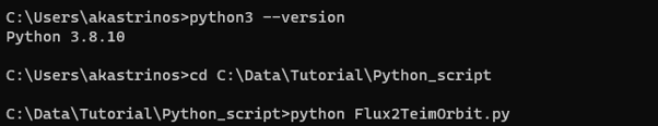
-
If the script is executed properly, you will receive the following
outputs:
- A printed message detailing the files used for the data extraction, thus the Torque Curve and Efficiency Map file names.
- A printed message ‘
File Output.efmp
                                    created
’. - The Output.efmp file saved in the script’s folder.
Figure 38. 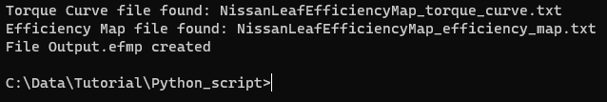
Note: The script searches for the result files with suffixes ‘_torque_curve.txt’ and ‘_efficiency_map.txt’. Therefore, you should not keep files from different motor models in the same directory or remove these suffixes from the file names. -
Once the directory is registered, enter python
Flux2TeimOrbit.py to execute the script, as shown
below:
- With the generated .efmp, you can now update the Dual Motor Electric Powertrain FMU with the new motor characteristic.
- (Optional) With Output.efmp motor file, return to Step 2 and enter the file as Motor properties file - front in the Motor Properties Dataset to change the electric vehicle’s front motor. Re-run the simulation to test the vehicle’s performance with the new electric motor.