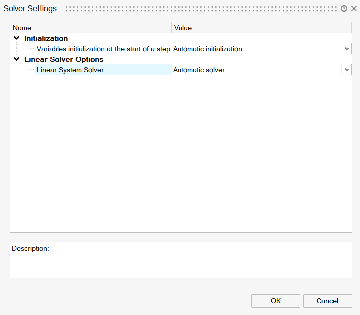
Solver Settings
![]()
The Solver Settings allow the user to set the Flux solvers options which will be taken by Flux (in batch) to solve the current solution.
Coefficient for circuit connected coils
- an electrical component of stranded coil conductor type defined in the circuit
- a coil geometrically defined entity to define the shape of coils
- from an electric point of view, there is only one electrical component
- from a geometric point of view, there is an "original" coil (the one described in the FE domain) and its "duplicates" by symmetry and/or periodicity
In this situation, the electrical component is a component that comprises several geometric coils.
- the coefficient CM, which takes into account the number and types of symmetries and/or periodicities
- the field Conductors in series or in parallel, which takes into account the configuration type of associated conductors (all in series, all in parallel).
In the Automatic mode which is suitable for most cases, the coefficient CM takes into account the number and types of symmetries and/or periodicities.
But it is possible to define manually the coefficient CM defined either as an integer or a fraction.
An example which needs a manual CM definition is a speed sensor defined with symmetry/periodicity, but the coils must not be duplicated. Then CM is defined by the value 1.
The 3 possible choices are explained in the table below:
| Option | Description |
|---|---|
| Automatic coefficient (symmetry and periodicity taken into account) | CM is automatically computed with taking active symmetries and active rotation periodicities of the problem into account. |
| Imposed coefficient (integer) |
CM is an integer: CM = N N is the number of repetitive patterns described in the finite elements domain (The finite elements domain corresponds to 1/N fraction of the real device) |
| Imposed coefficient (fraction) |
CM is a quotient of 2 integers: CM = N1/N2 The finite elements domain corresponds to 1/N1 fraction of the real device. N1 is the number of repetitive patterns described in the finite elements domain N2 is the number of repetitive patterns supplied by the electric circuit |
Complete cuts automatically
When magnetic bodies have hole(s), magnetic cuts may be required to have good results.
When this option is enabled (default choice), at solve, Flux executes the automatic cuts creation algorithm before running the Flux solving.
For more information, please check Automatic Cuts creation for 3D Magnetostatic solution
Initialization
Variables initialization at the start of a step
This option concerns the initialization of the state variables at the start of a step.
- Transient solutions
- Static and AC solutions with Motion load and constraint
- With zero solution
Robust for non-linear convergence
- With the previous step solution (by
default)
Faster, but can impact the non-linear convergence
- With a predicted solution
Recommended for hysteretic materials.
Linear Solver Options
A linear system of n equations and n unknowns can be written under the following matrix form:
AX=B
- A is a square matrix of n x n size (with n lines and n columns)
- X is a column vector of size n, representing the system unknowns
- B is a column vector of size n, with known components
To find the solution, i.e. the vector X, a linear solver must be employed. Two types of solvers can be distinguished: the Direct and Iterative solvers.
The Direct solvers follow a process that leads to a very accurate solution but at the cost of several time and memory-expensive operations for large problems.
The Iterative solvers follow an iterative process that approximates a solution at each iteration. Usually, the process tends to provide a solution closer to the real solution of the linear system from iteration to the next. The process comes with a stopping criterion, depending on the accuracy threshold set for the approximated solution and the maximal number of iterations. Thus, the Iterative solver can lead to faster solutions and lower memory consumption for large problems but can be less accurate.
The linear solver is used in all EM solutions.
| Dimension | 2D | 3D | |||
|---|---|---|---|---|---|
| Solution | Any | Others | Magnetostatic Integral method | Steady-state AC | |
| Number of nodes | Any | < 500,000 | > 500,000 | Any | Any |
| Solver | Direct | Direct | Iterative | Iterative | Direct |
- For HPC (High Performance Computing) hardware or computers with a great amount of RAM, the Direct solver will be the most suitable choice thanks to its scalability and parallel potential.
- For computers with a low amount of RAM, it would be more advisable to use the Iterative solver for its low memory consumption.
- For 2D problems, the number of unknowns is relatively low, thus Direct solver should deliver better results in terms of solving time.
This section targets advanced users and wants to help understand what solver parameters do. Here are the solver options for Direct and Iterative solvers:
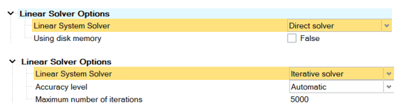
The Direct solver option available consists in using the disk for the solving in addition to the RAM. This option is very useful since it allows extending the amount of usable memory. However, using the disk implies slower operations since disks are significantly slower to compute i/o operations. If the disk memory usage is checked and no directory is selected, the default scratch directory is taken.
On the right-hand side figure, two options are displayed for the Iterative solver: the precision level (or threshold) and the maximal number of iterations. The automatic accuracy level is based on the problem type. It is possible to select a High accuracy level to ensure the result quality but it will lead to slower computation. The maximal number of iterations field allows to set a limitation on the solving time. Increasing the value can lead to more accurate results but with slower computation. Reducing the value can lead to faster computation but with reduced accuracy.