Force Computation
![]()
Solution coupling (2D/3D Transientmagnetics → Modal Frequency Response / E-Motor Acoustic)
Description
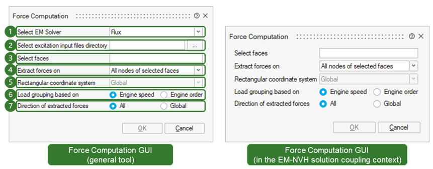
This tool is used to compute excitation loads on the selected faces (stator teeth, rotor part, or both of them) of a motor using an EM solver and automatically set up LoadCase of modal frequency response analysis for OptiStruct.
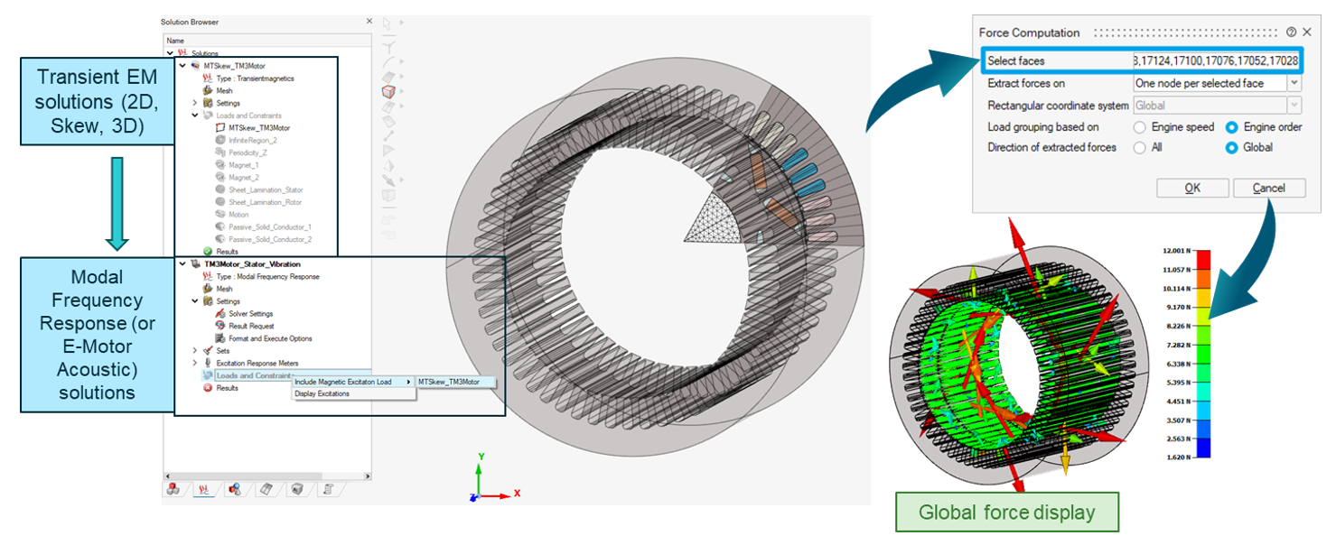
The GUIs of the force computation tool are shown below: as a general tool (left); in the EM-NVH solution coupling context (right):
Force computation process
The Force Computation tool supports the two EM solvers (1) below:
- Flux
- JMAG
This document will focus on the case where the EM solver is Flux.
If the Flux is selected as the electromagnetic force computation solver, the user needs to specify the content:
- Flux project directory (2)
- Specify the 2D, Skew or 3D transient magnetic project (*.FLU folder) which is already solved using Altair Flux.
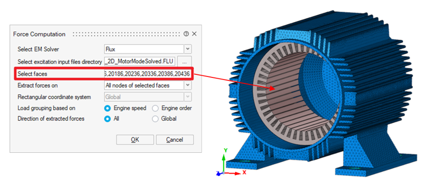
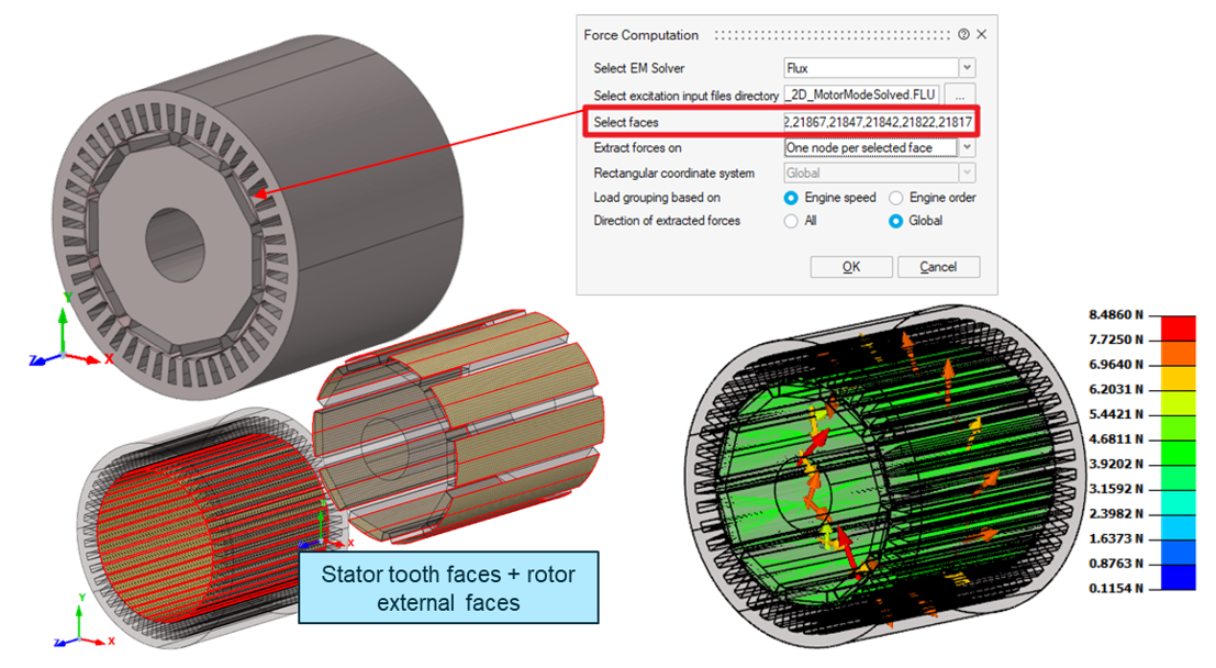
- Select the faces to perform force computation as inputs (3). All faces used for
force computation can be selected directly in the working area, as shown below:
- EM forces can be extracted in the following two approaches (4), as shown in the
next image.
- All-node approach - Excitation load will be computed for all the nodes in the selected faces, as nodal forces.
- One-node-per-face approach - Only one excitation load will be
computed at the centroid of each selected face. The connection between each
node and this global force is realized through RBE3.
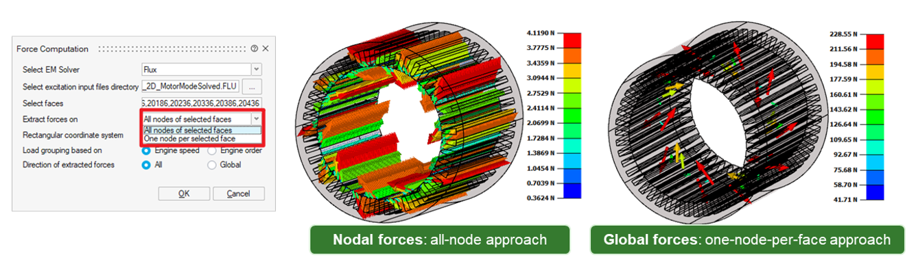
Note: The final NVH analysis results of the electromagnetic forces calculated based on these two approaches are similar. However, by using global forces, the file size and the response time of reading the Database can be reduced. -
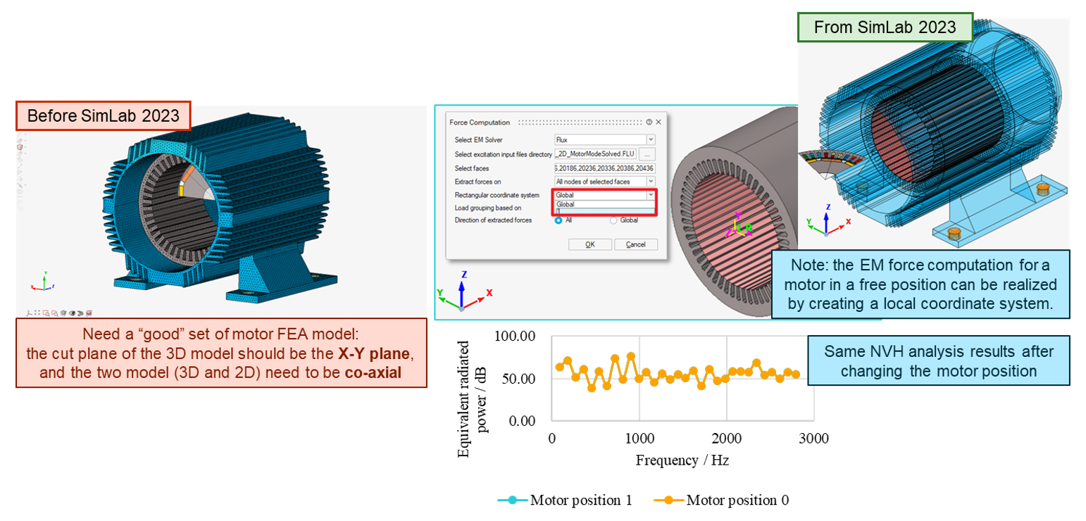
The additional coordinate system (5) can be used to compute EM forces for a 3D NVH model not well aligned with the 2D EM model. Previously (before the SimLab 2023), the cut plane of the 3D NVH model need to be the X-Y plane (Flux 2D project working plane), and both models (3D and 2D) need to be co-axial. By defining an additional coordinate system (which is created for the local stator tooth face local expression), the EM forces can be also computed for a 3D model which is in a free place.
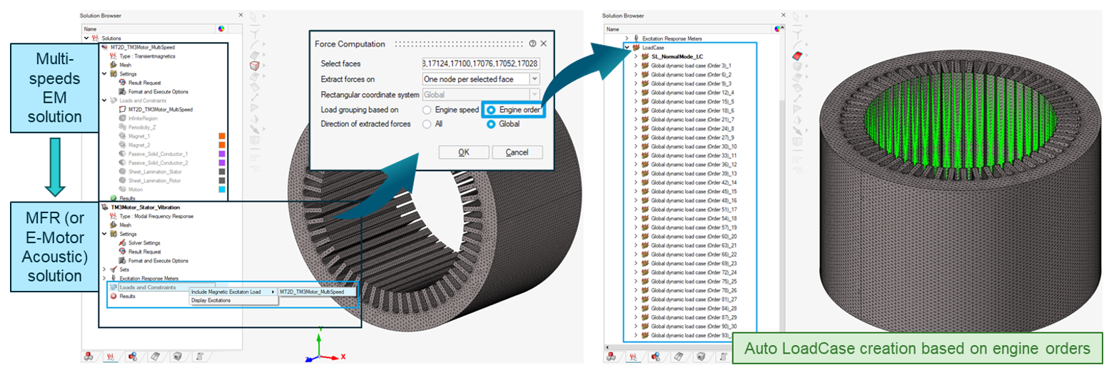
- Excitation load computed from the Flux can be grouped based on two methods
(6):
- Engine Speed - The excitation loads are grouped based on the engine speed.
- Engine Order - The excitation loads are grouped based on the
frequency (order) across all available speeds.Note: The Engine Order option works only for an EM project input with multiple working point results (multi-speed analysis).
- Excitation load computed from the Flux can be selected the required component (7)
to import in SimLab:
-
All - the computed force results will be converted as multiple LoadCase:
Global – resulting forces
First component – radial component
Second component – tangential component
Third component – moment (only for the global forces)
-
Global - the computed force results will be converted to a single LoadCase:
Global – resulting forces

-
Things to note
-
SimLab supports a direct coupling of a Modal Frequency Response or an E-Motor Acoustic solution with a transient EM solution (2D, Skew or 3D). Once the EM solution gets solved, it can be used for the force computation in the following solution setting, as shown below:
-
During the force computation process, SimLab will call Flux in the background where the actual computation takes place. Once the force computation process is finished, the force file (.FEM) will be automatically converted as the SimLab LBCs (PointForce and ExcitationLoad).
Note: Users can also import an electromagnetic force file (*.FEM) exported from the Flux I/E context into Simlab. And the file can be also automatically convert to SimLab LBCs, as shown below: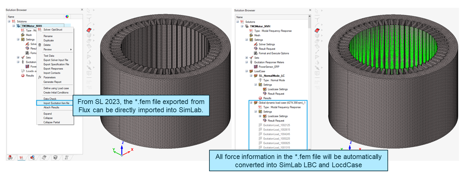
-
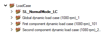
Based on excitation load information, modal frequency response analysis LoadCases will be created in SimLab. If the 2D electromagnetic project involves multi-speed analysis results, SimLab will create for each speed value a LoadCase and continue to perform the multi-speed EM-NVH analysis, as shown below:
Note: Multi-speed analysis built on SimLab-EM is perfectly compatible with the force computation tool. If the multi-speed analysis is done in the Flux Legacy version, please make sure that the motor speed parameter is named "SPEED". - Modal frequency LoadCases will refer to a normal mode LoadCase. If normal mode LoadCase is not available, it will be created and referred in modal frequency LoadCases.
- For One-node-per-face approach: Additional Load case will be created for each speed to include the moments.
-
During this process Load case settings for all load cases will be created automatically to extract eigen mode value for the structure and fluid and forcing frequencies.
- The fluid mode extraction will be done only if the solution includes fluid bodies.
-
Simlab supports displaying all computed electromagnetic forces (in the frequency domain).
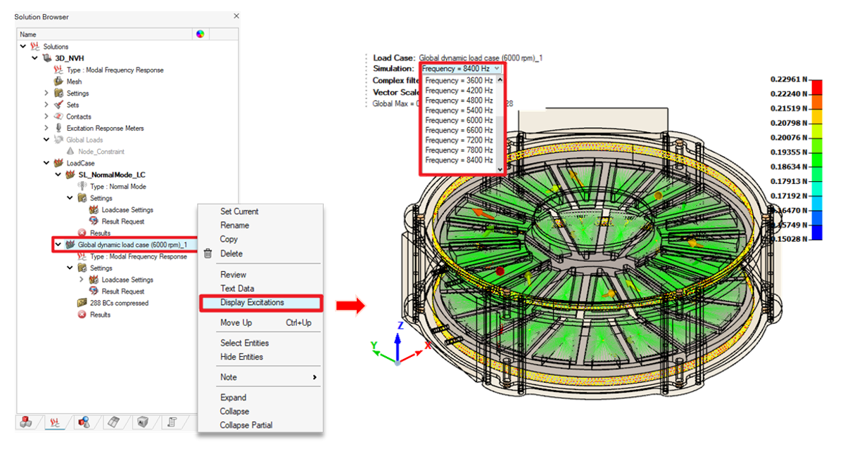
-
Starting from SimLab 2025.1, it is possible to simultaneously compute the electromagnetic forces in different regions (stator and rotor) of a motor and convert them into SimLab LBCs.
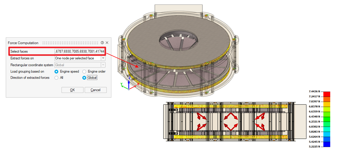
-
Starting from SimLab 2025.1, it is possible to compute the electromagnetic forces from a 3D motor (e.g. axial flux machines) and convert them into SimLab LBCs.
-
Frequency step value and cutoff frequency of the electromagnetic excitation
Since the electromagnetic force computation process involves converting the force results from the time domain to the frequency domain (via FFT operation), it is necessary to have a certain understanding of the frequency step value and cutoff frequency of the obtained results.
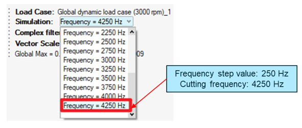
-
Frequency step value: Different from the mechanical fundamental frequency (motor speed in RPM / 60) during motor rotation, the frequency step value of the results depends on the number of electrical periods that have been taken into account in the EM simulation.
-
Example: For a motor with 5 pole pairs, one electrical cycle is 360 / 5 = 72 degrees. Thanks to periodicity, from the perspective of EM analysis, only one electrical cycle is enough to be simulated to reconstruct the results of a full cycle (360 degrees). In this case, the frequency step value will be motor speed in RPM / 60 *5.
-
-
Cutoff frequency: When computing the FFT of a force signal, the computed harmonics are valid up to the cutting frequency. Beyond this limit, the computed harmonics are no longer valid and represent numerical noise.
The cutoff frequency is defined as the frequency for which the wavelength discretization is 4 points per wavelength. And the cutoff frequency will not be represented in the force results.
-
Example: For a motor operating at 1080 RPM, if the simulation is angle-controlled (angle step is 1 degree), the time step can be calculated as
TimeStep = AngleStep/(SpeedRPM/60*360) = 0.00015432 s
Then the cutoff frequency can be obtained as
F_c = 1/(4*TimeStep) = 1620 Hz
-
-