RD-E: 1600 Dummy Settling

Quasi-static loading analysis on a dummy, settling on a seat before crash analysis, using Altair Radioss explicit or Radioss implicit solvers.

The topic of this study concerns quasi-static load treatment of dummy settling using different approaches to check the convergence speed and results accuracy.

Standard explicit method with constant loading,
Explicit method with kinetic relaxation (/KEREL)
Explicit with dynamic relaxation (/DYREL)
Explicit with dynamic relaxation with auto-defined adaptive damping (/ADYREL)
Explicit with Rayleigh damping (/DAMP)
Nonlinear implicit solution (/IMPL)

Options and Keywords Used

Units used: Mg, mm, s

/SHELL,/BRICK, and /BEAM elements
Quasi-static analysis by explicit, kinetic and dynamic relaxation (/KEREL, /DYREL and /ADYREL), and Rayleigh damping (/DAMP)
Contact interface (/INTER/TYPE7)
Hyperfoam material (/MAT/LAW62 (VISC_HYP))
Linear elastic material (/MAT/LAW1 (ELAST))
General solid property set (/PROP/TYPE14 (SOLID)) and shell property (/PROP/TYPE1 (SHELL))
Void material (/MAT/LAW0 (VOID)) and void property (/PROP/TYPE0 (VOID))
Added mass (/ADMAS)
Boundary conditions (/BCS)
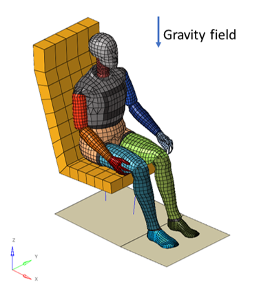
Gravity (/GRAV)
Rigid body (/RBODY)

Input Files

Before you begin, copy the file(s) used in this example to your working directory.

Explicit: RD-E-1601_Explicit.zip
Implicit: RD-E-1602_Implicit.zip

Model Description

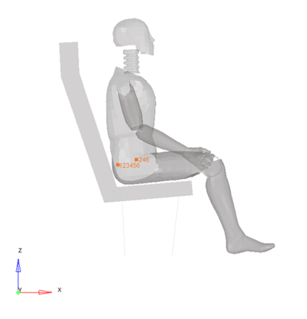
Model Method

The model consists of two subsets:

a dummy with only the external surface is defined as a rigid body
a seat is comprised of six parts:
- foam seat back
- foam seat cushion
- seat back brace
- seat bottom brace
- seat legs
- the floor

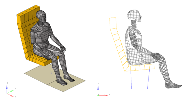
The goal is to settle the dummy on the seat using a quasi-static approach to obtain static equilibrium. For this example, the dummy’s limbs are already positioned at the desired position before the gravity load is applied.

The seat structure and the floor are defined in a rigid body. Only the seat cushion parts are deformable during simulation.

The main node coordinates, and skew are extracted from the pelvis part of the dummy rigid body.

Gravity is applied to all nodes of the model. A function defines gravity acceleration in the Z-direction versus time. The gravity is activated by using the /GRAV keyword in the Starter file (*_0000.rad).

The main node of the seat and floor rigid body is clamped.

The main node of the dummy model rigid body is free to translate along X and Z axis and rotate around Y axis.

Material Properties

Material for seat support - both the legs and the floor are made of steel with the following properties (/MAT/LAW1):

Material Properties: Value
Young's modulus: 210000 $[MPa]$
Poisson's ratio: 0.3
Density: 7.8E^-9 ton/mm³

The seat cushion is made of foam which can be described using hyperfoam model (/MAT/LAW62), with the following properties:

Material Properties: Value
Ground shear modulus: (0.02,2), (0.01,-2)
Poisson's ratio (foam behavior): 0
Density: 7.8 x 10^-9 ton/mm³

The dummy model parts are void material (/MAT/VOID). The material properties are used to compute the contact stiffness:

Material Properties: Value
Young's modulus: 2070 $[MPa]$
Poisson's ratio: 0.28
Density: 5E^-11 ton/mm³

Element Properties

The seat cushion is meshed with 70 brick elements defined by general /PROP/TYPE14 solid property.

I_solid: 24 (HEPH)
I_cpre, I_frame and I_smstr: Set to -1 (Recommended value)

The other parameters are set to default (0).

The seat structure and the floor are modeled with shell elements defined in the rigid body:

Seat back thickness: 2 mm
Floor thickness: 1 mm

Shell properties used are default value for all parameters (0).

The seat legs have the following characteristics:

Area

2580 mm²

Inertia

IXX: 554975 mm⁴
IYY: 554975 mm⁴
IZZ: 937908 mm⁴

Void property (/PROP/TYPE0 (VOID)) is used for the dummy’s components. The thickness is used compute the contact stiffness:

Dummy thickness: 1 mm

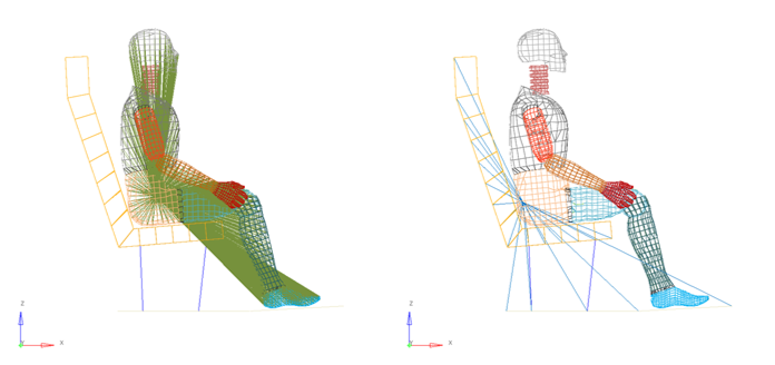
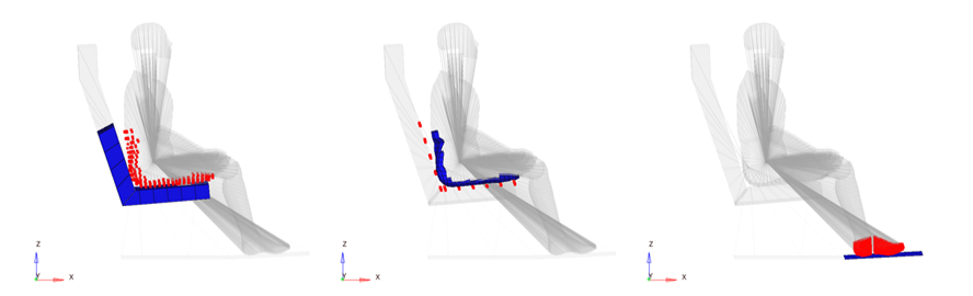
Contact Interfaces

Seat foams define the Main surface, Dummy parts define the Secondary nodes
Dummy parts define the Main surface, Seat foams define the Secondary nodes (symmetrical contact)
The floor defines the Main surface, dummy feet define the Secondary nodes

The contact interfaces use the following parameters:

Contact gap: 5 mm
Coulomb friction: 0.3
Stiffness: 4 (minimum stiffness between main and secondary)
Minimum stiffness: 1000 N/mm (usually value for automotive crash analysis)
Friction formulation: 2 (stiffness)

Refer to the Radioss Theory Manual and Starter Input for further information about the definition of the TYPE7 interface.

Resolution Methods

Quasi-static treatment of gravity loading up to equilibrium using:

Explicit solver:
A quasi-static simulation using a dynamic resolution method needs to minimize the dynamic effects to converge towards static equilibrium. This usually describes the pre-loading case prior to dynamic analysis. Thus, the quasi-static solution of gravity loading on the model is the steady-state part of the transient response.

A first analysis is done to view the dynamic effect due to gravity loading and compare the results with the different methods to reduce the dynamic effect.
To reduce the dynamic effect, the following options are available in the Engine file:
- Kinetic energy relaxation (/KEREL)
  All velocities are set to zero each time the kinetic energy reaches a maximum value (no additional input parameters are required).
- Dynamic relaxation (/DYREL)
  - Dynamic relaxation with a user-defined damping factor and period to damp.
  - The model without dynamic relaxation is computed to identify the period to damp and defined the parameters for the /DYREL card.
- Dynamic relaxation (/ADYREL)
  - Dynamic relaxation with auto-defined adaptive damping.
  - Radioss solver automatically defines the period to damp. There is no parameter to set.
- Rayleigh damping (/DAMP)
  - Rayleigh mass and stiffness damping coefficients applied to a set of nodes for any nodal DOF either in local or global coordinate system.
  - For this application, the mass needs to be damped to reduce the kinetic energy.
  - The parameter, $α$ is defined as a damping percentage divided by the computation time step.
Detailed information about the different formulations are available in the Radioss Theory Manual.
Implicit solver:
However, the implicit algorithm uses a global resolution which requires convergence for each time step and has low robustness in comparison to the explicit (null pivots, divergence for high nonlinearities, and so on).

The implicit methods result in solving a linear system for each time step, which is relatively expensive but enables a large time step: so there are few expensive calculations. The explicit method treats linear or nonlinear systems depending on the problem. It is less expensive and faster for each step, but requires short time steps to ensure stability of the scheme that has many inexpensive cycles.

For this example, the following implicit solution and solver is used:

Nonlinear solver

Modified Newton method with relative residual in force (/IMPL/NONLIN/1)

Linear solver

Direct solver MUMPS (/IMPL/SOLVER/2)

Quasi-static solution

Considers the mass and inertia with a scale factor (/IMPL/QSTAT/DTSCAL)

Time step

Arc-length method is used to accelerate and to control the convergence (/IMPL/DT/2)

Time step control

Initial (/IMPL/DTINI), minimum and maximum time step (/IMPL/DT/STOP)

Detailed information about the different formulations are available in the Radioss Theory Manual.

Results

Curve and Animation

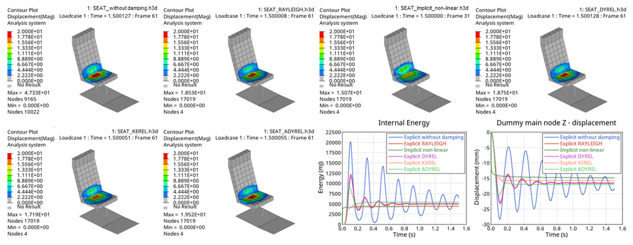
The results are similar for all methods used; except for the model without relaxation or damping (as is to be expected).

The different methods show different convergence time.

Model: Convergence time
Explicit without damping: Can not converge to static equilibrium
Explicit ADYREL: 0.4
Explicit DYREL: 1.5
Explicit KEREL: 0.2
Explicit RAYLEIGH: 1.5
Implicit Nonlinear: > 1.5

Conclusion

The model with dynamic relaxation (/DYREL), automatic dynamic relaxation (/ADYREL), and Rayleigh damping (/DAMP) converges to the same results. Automatic dynamic relaxation converges faster.

The results can be slightly different between the methods mainly because of the contact treatment, how the contact starts and how it evolves according to the elastic vibrations.