RD-E: 0800 Hopkinson Bar

The purpose of this example is to model and predict the responses of very high strain rates on a material during impact.

High strain rate characterization of 7010 aluminum alloy using Split-Hopkinson pressure bar experiment.

Precise data for high strain rate materials is necessary to enable the accurate modeling of high-speed impacts. The high strain rate characterization of materials is usually performed using the Split-Hopkinson pressure bar within the strain rate range 100-10000 s^-1. It is assumed that during the experiment the specimen deforms under uniaxial stress, the bar specimen interfaces remain planar at all times, and the stress equilibrium in the specimen is achieved using travel times. The Radioss explicit finite element code is used to investigate these assumptions.

Options and Keywords Used

Units used: g mm s MPa

/QUAD: 2D solid elements defined in the global YZ – plane
/ANALY: Defines the type of analysis and sets analysis flags
/MAT/LAW1 (ELAST): Isotropic, linear elastic material using Hooke's law
/MAT/LAW2 (PLAS_JOHNS): Isotropic elasto-plastic material using the Johnson-Cook material model
/PROP/TYPE14 (SOLID): General solid property set
/IMPVEL: Imposed velocities on a group of nodes
/BCS: Boundary conditions)

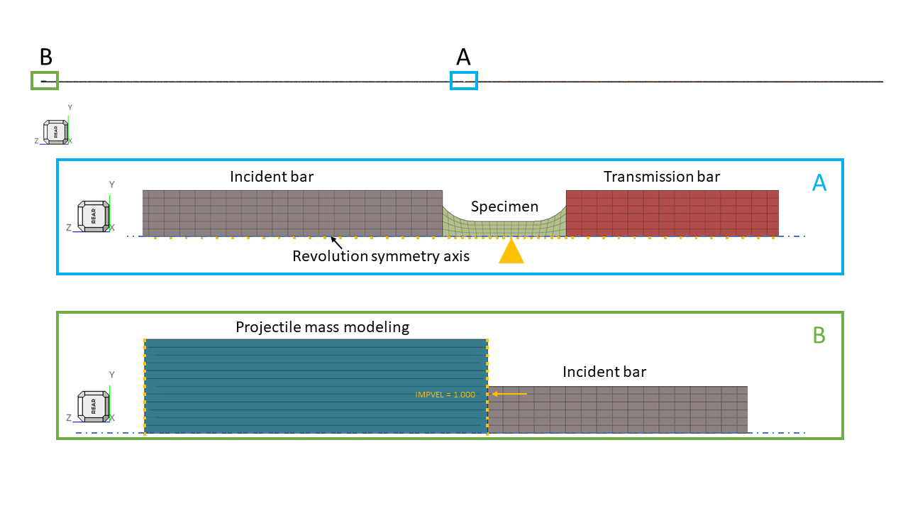
Low extremity nodes of the output bar are fixed in the Z direction. The axisymmetric condition on the revolutionary symmetry axis requires the blocking of the Y translation and X rotation.

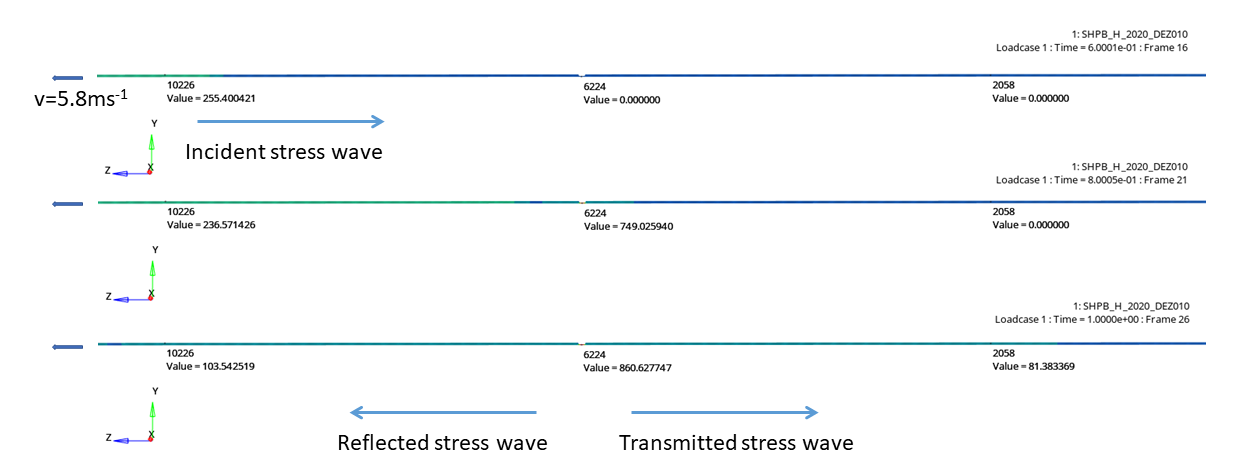
The projectile is modeled using a steel cylinder with a fixed velocity in the direction Z. The required strain rate is considered by applying two imposed velocities, 1.7 ms^-1 and 5.8 ms^-1 in order to produce strain rates in the ranges of 80 s^-1 and 900 s^-1 (low and high rates).

True Stress, True Strain and True Strain Rate Measurement from Time History

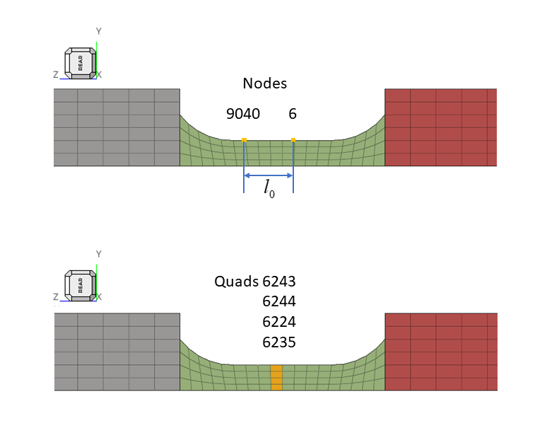
In the experiment, the strain gauge is attached to the specimen. In simulation, the true strain will be determined from 9040 and 6 nodes’ relative Z displacements ( $l_{0}$ = 3.83638 mm).

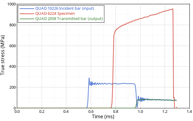
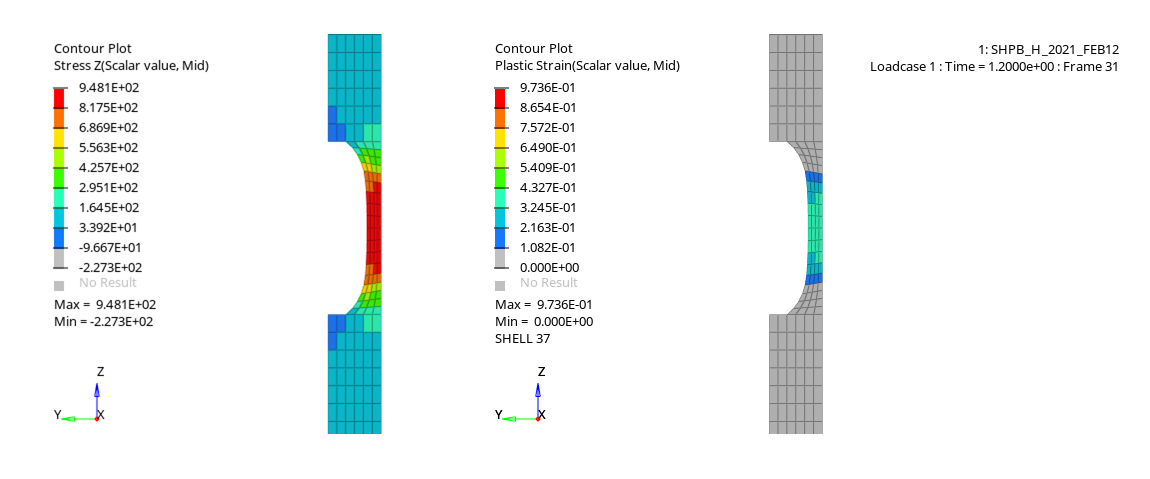
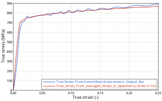
The true stress can be given using two data sources. The first methodology consists of using the equation previously presented, based on the assumption of the one-dimensional propagation of bar-specimen forces. The engineering strain $ε_{t}$ associated with the output stress wave is obtained from the Z displacement of nodes located on the output bar. The true plastic strain is extracted from the quads on the specimen, saved in the Time Histories file. True stress can also be measured directly from the Time History using the average of the Z stress quads 6243, 6244, 6224 and 6235. It should be noted that the section option is not available for quad elements.

The strain rate can be calculated from either the true plastic strain of quads saved in /TH/QUAD or from the true strain

ε_{true}

Table 1. Relations Used in the Analysis
	High Rate Testing
True stress	$σ_{t r u e} (t) = \frac{S_{b a r} E_{b a r}}{S_{s p e c i m e n}} ε_{T} (t) \exp (ε_{p l} (t))$	Z stress average from quads saved in /TH
True strain	$ε_{t r u e} (t) = \ln (\frac{l_{i} (t)}{l_{0}}) l_{i} (t) = l_{0} + Δ l = l_{0} + (u_{9040} (t) - u_{6} (t))$
True strain rate	$\dot{ε} = \frac{Δ ε_{p l} (t)}{Δ t}$	$\dot{ε} = \frac{Δ ε_{t r u e} (t)}{Δ t}$

Input Files

Before you begin, copy the file(s) used in this example to your working directory.

RD-E-0800_Hopkinson_bar.zip

Model Description

The purpose of this example is to model and predict the responses of very high strain rates on a material during impact.

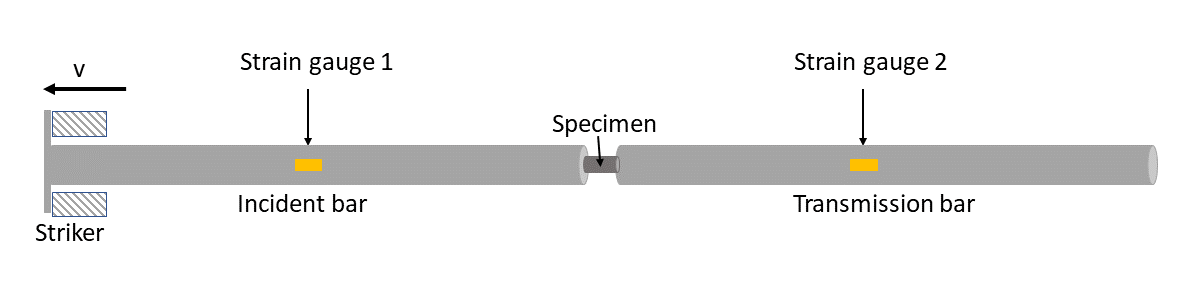
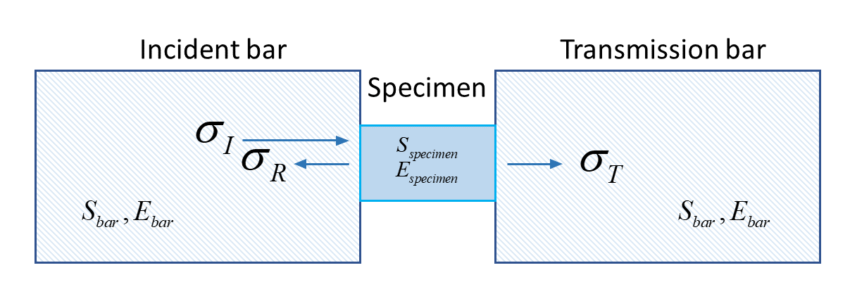
The Split-Hopkinson pressure bar is a suitable method to perform experiments with high strain rates.

Figure 3 shows the principal test setup, consisting of:

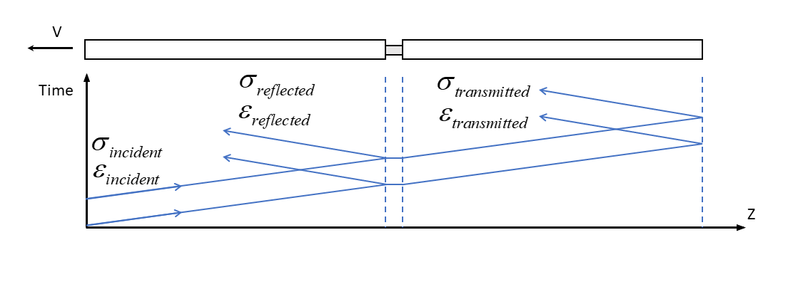
an incident bar and a transmission bar of equal length, between which the sample to be tested is clamped.
a striker is attached to the outer end of the incident bar. When a steel projectile hits the striker, a stress pulse is introduced into the incident bar.

The impact generates a strain (tensile) wave which propagates through (along) the Incident bar and is detected by strain gauge 1. Part of the wave is reflected, and a part is transmitted via the specimen’s interface. So, the stress pulse continues through the specimen and into the transmitted bar. Strain gauges 1 and 2 are attached to the incident bar and transmission bar to detect the strain wave signal. The wave reflections inside the sample enable the stress to be homogenized during the test. The strain associated with the output or transmitted stress wave is measured by the strain gauges on the output or transmitted bar. The strain gauges attached to the specimen gauge length provide direct measuring of the true strain and the true plastic strain in the specimen during the experiment. The transmitted elastic wave provides a direct force measurement to the bar specimen interfaces by way of the following relation.

(1)

F (t) = S_{b a r} \cdot E_{b a r} \cdot ε_{T} (t)

Where,

$E_{b a r}$: Modulus of the output bar.
$ε_{T}$: Strain associated with the output stress wave.
$S_{b a r}$: Cross-section of the output bar.

If the two bars remain elastic and wave dispersion is ignored, then the measured stress pulses can be assumed to be the same as those acting on the specimen.

The engineering stress value in the specimen can be determined by the wave analysis, using the transmitted wave:(2)

σ_{e n g i n e e r i n g} (t) = \frac{F (t)}{S_{s p e c i m e n}} = \frac{S_{b a r} E_{b a r}}{S_{s p e c i m e n}} ε_{T} (t)

Engineering stress can also be found by averaging out the force applied by the incident that is the reflected and transmitted wave, as shown in the equation:(3)

σ_{e n g i n e e r i n g} (t) = \frac{S_{b a r} E_{b a r}}{2 S_{s p e c i m e n}} [ε_{l} (t) + ε_{R} (t) + ε_{T} (t)]

Where,

$ε_{I}$ and $ε_{R}$: Strains associated with input stress wave.
$ε_{T}$: Strain associated with output stress wave.

True stress in the specimen is computed using the following relation (refer to RD-E: 1100 Tensile Test for further details):(4)

σ_{t r u e} = σ_{e n g i n e e r i n g} \exp (ε_{t r u e})

The true strain rate is given by:(5)

\dot{ε} = \frac{Δ ε_{t r u e}}{Δ t}

True stress and true strain are evaluated up to the failure point.

Interface 1: $F_{1} = S_{b a r} [σ_{l} (t) + σ_{R} (t)] = S_{b a r} \cdot E_{b a r} [ε_{l} (t) + ε_{R} (t)]$
Interface 2: $F_{2} = S_{b a r} \cdot σ_{T} (t) = S_{b a r} \cdot E_{b a r} \cdot ε_{T} (t)$
Balance in specimen: $F_{1} = F_{2}$ ; $ε_{l} (t) + ε_{R} (t) = ε_{T} (t)$
Engineering stress in specimen: $σ_{s p e c i m e n} (t) = \frac{F_{1}}{S_{s p e c i m e n}} = \frac{F_{2}}{S_{s p e c i m e n}}$

Strain Rate Filtering

Because of the dynamic load, strain rates cause high frequency vibrations which are not physical. Thus, the stress-strain curve may appear noisy. The strain rate filtering option enables to dampen such oscillations by removing the high frequency vibrations in order to obtain smooth results. A cut-off frequency for strain rate filtering F_cut = 30 kHz was used in this example. Refer to RD-E: 1100 Tensile Test for further details.

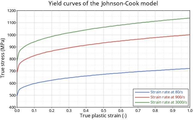
Johnson-Cook Model

The Johnson-Cook model describes the stress in relation to the plastic strain and the strain rate using the following equation:(6)

σ = \underset{\begin{array}{l} Influence of \\ plastic strain \end{array}}{\underset{︸}{(a + b ε_{p}^{n})}} \underset{\begin{array}{l} Influence of \\ strain rate \end{array}}{\underset{︸}{(1 + c \ln \frac{\dot{ε}}{{\dot{ε}}_{0}})}}

Where,

$\dot{ε}$: Strain rate.
${\dot{ε}}_{0}$: Reference strain rate.
$ε_{p}$: Plastic strain (true strain).
$a$: Yield stress.
$b$: Hardening parameter.
$n$: Hardening exponent.
$c$: Strain rate coefficient.

The two optional inputs, strain rate coefficient and reference strain rate, must be defined for each material in /MAT/LAW2 in order to take account of the strain rate effect on stress, that is the increase in stress when increasing the strain rate. The constants $a$ , $b$ and $n$ define the shape of the strain-stress curve.

In the documents entitled CRAHVI, G4RD-CT-2000-00395, D.1.1.1, Material Tests – Tensile properties of Aluminum Alloys 7010T7651 and AU4G Over a Range of Strain Rates, the behavior of the 7010 aluminum alloy can be described according to the relations:

$σ = (496 + 225 ε^{0.35})$: Strain rates below 80 s^-1
$σ = (496 + 225 ε^{0.35}) (1 + 0.16 \ln (\frac{\dot{ε}}{0.08}))$: Strain rates exceeding 80 s^-1 up to 3000 s^-1

The material properties of the specimen are:

Material Properties: Value
Young's modulus: 73000 $[MPa]$
Poisson's ratio: 0.33
Density: 0.0028 $[\frac{g}{m m^{3}}]$

The material used for the bars and projectile is TYPE1 (linear elastic) with the following properties:

Material Properties: Value
Young's modulus: 210000 $[MPa]$
Poisson's ratio: 0.33
Density: 0.0078 $[\frac{g}{m m^{3}}]$

The geometrical characteristics of the bars and projectile are:

Bars
Length: 4 m
Diameter: 12 mm

Projectile
Radius: 12 mm
Weight: 170 g

Model Method

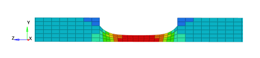
Considering the geometry’s revolution symmetry the material and the kinematic conditions, an axisymmetric model is used (N2D3D = 1 in /ANALY set up in the Starter file). Y is the radial direction and Z is the axis of revolution.

The mesh is made of 12054 2D solid elements (quads). The quad dimension is about 2 mm.

Results

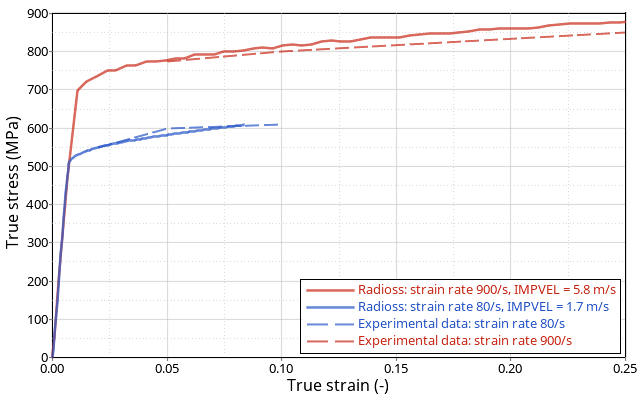
The purpose of the test is to obtain results at high deformation rates. In this model the Johnson-Cook type material law is used. The increase of stress is expected to be approximately 30% above the stress compared to the quasi-static deformation rate.

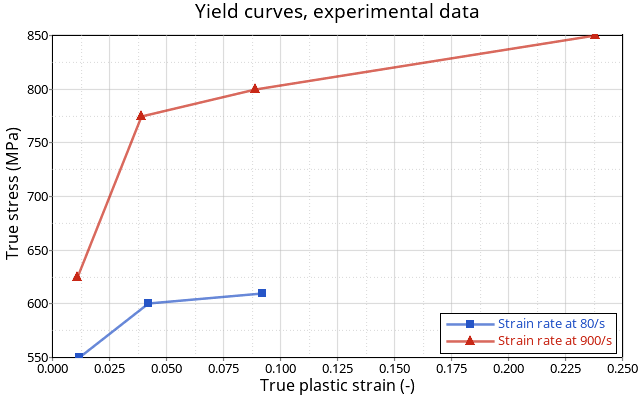
Experimental Data

Experimental results show that the variation of the true tensile flow stress compared with the true strain is approximately equivalent to a strain rate between 80 s^-1 and 100 s^-1. The reference strain, $ε_{R}$ in the Johnson-Cook model is set to 0.08 ms^-1 (correspond to 80 s^-1, which represents the quasi-static deformation rate. At higher deformation rates, the true flow stress increases significantly with increasing strain rates. The 7010 aluminum alloy exhibits an increase in the flow stress by a typical value of 30% at high strain rates (900 s^-1 – 3000 s^-1) compared to the quasi-static value.

Results are given at the specific true strains of 0.02, 0.05 and 0.10. The influence of the strain rate on the stress can be seen in Figure 8. ¹

For the test performed with a strain rate of 900 s^-1, the flow stress reaches 850

[MPa]

at a 0.25 strain.

Table 2. True Stress at Specific Strains using Both Strain Rates (experimental data)
	Strain Rate: 80 s^-1			Strain Rate: 900 s^-1
True strain	0.02	0.05	0.1	0.02	0.05	0.1	0.25
True plastic strain	0.012	0.042	0.092	0.011	0.039	0.089	0.238
True stress (MPa)	550	600	610	625	775	800	850

Johnson-Cook Model

Figure 9 shows the variation of true stress in time in relation to the wave propagation along the bars. Stresses are evaluated on the input bar, the specimen and the transmission bar.

The stress-time curve shows the incident, reflected and transmitted signals.

The speed of wave,

C

along the bars is calculated using the relation:(7)

C = \sqrt{\frac{E}{ρ}} = 5189 m s^{- 1}

Where,

$E$: Young's modulus.
$ρ$: Density of the bars.

The time step element is controlled by the smallest element located in the specimen. It is set at 5x10^-5 ms. The stress wave thus reaches the specimen in 0.77 ms and travels 0.26 mm along the bar for each time step. Obviously, it remains lower than the element length of the smallest dimension (0.88 mm).

An imposed velocity of 5.8 ms^-1 produces a strain rate in the specimen of approximately 900 s^-1, while a strain rate of approximately 80 s^-1 is achieved using an imposed velocity of 1.7 ms^-1. A simulation is performed for each velocity value.

Note: The study on low rates is more limited in time than on high rates due to the reflected wave generated on top of the output bar.

Figure 13 shows the true stress and true strain as a function of the strain rate.

At a high strain rate (900/s), an increase in the flow stress is observed, being approximately 30% higher than the stress obtained for a low strain rate (80/s). The Johnson-Cook model used provides precise results compared with the experimental data.

The true stresses determined from both methodologies are shown side-by-side. This validates the analysis based on a transmitted wave. Typical curves for a model having imposed velocities equal to 5.8 ms^-1 (Figure 15 and Figure 16).

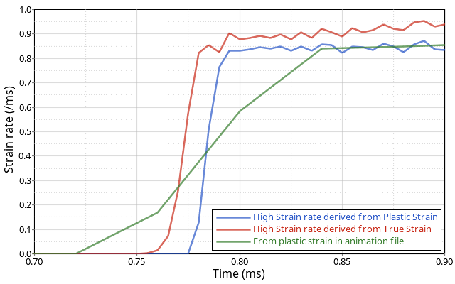
Either data sources used to evaluate the strain rate give similar results.

The results show:

the strain rate effect on stress, with or without the cut-off frequency for smoothing (100 kHz);
the influence of the strain rate coefficient (comparison with experimental data).

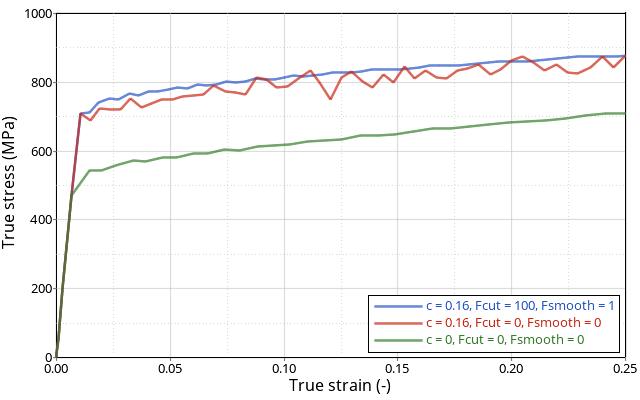
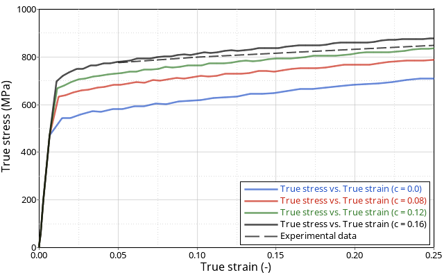
These studies are performed for the high strain rate model ( $ε$ = 900 s^-1).

Figure 19 compares the distribution of the von Mises stress on the specimen, with and without the strain rate filtering at time t=0.88 ms.

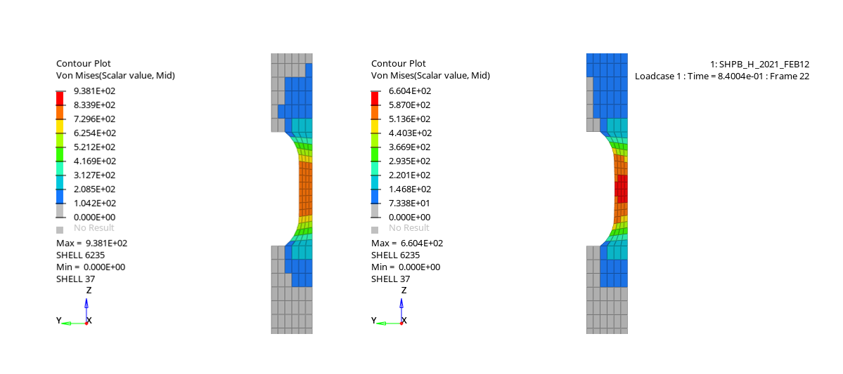
More physical flow stress distribution is obtained using filtering. Explicit is an element-by-element method, while the local treatment of temporal oscillations puts spatial oscillations into the mesh.

¹ CRAHVI, G4RD-CT-2000-00395, D.1.1.1, Material Tests - Tensile properties of Aluminum Alloys 7010T7651 and AU4G Over a Range of Strain Rates.