
Exercise 2: Nonlinear Gap Analysis
Create Load Step Inputs Defining Parameters
- In the Model Browser, right-click and select .
- For Name, enter nonlinear.
-
For Config type, select Nonlinear Parameters.
The default for Type is NLPARM.
-
Click NINC and enter 10.
NINC denotes the number of load sub-increments. If NINC is blank, then the entire loading is applied at once. An NINC of 10 signifies that the load will be sub-divided into 10 equal increments.
- Click MAXITER and leave the default value of 25.
-
For error tolerances EPSU, EPSP, and EPSW, enter 0.001,
0.001, and 1e-07
respectively.
For details on these tolerances, refer to the Nonlinear Quasi-static Gap and Contact Analysis section in the online help.
Figure 1. 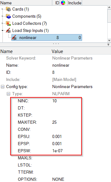
Update the Load Steps
- Open the Load Step folder in the Model Browser.
- Click the Coup_Vert load step to open the Entity Editor.
- For NLPARM, click .
-
In the Select Load step input dialog, select the
nonlinear load step inputs and click
OK.
Figure 2. 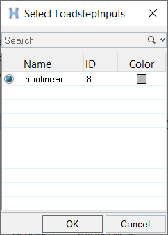
- Repeat this process for the Pressure load step.
Submit the Job
-
From the Analysis page, click the OptiStruct
panel.
Figure 3. Accessing the OptiStruct Panel 
- Click save as.
-
In the Save As dialog, specify location to write the
OptiStruct model file and enter
rib_nonlinear for filename.
For OptiStruct input decks, .fem is the recommended extension.
-
Click Save.
The input file field displays the filename and location specified in the Save As dialog.
- Set the export options toggle to all.
- Set the run options toggle to analysis.
- Set the memory options toggle to memory default.
- Click OptiStruct to launch the OptiStruct job.
The default files written to the directory are:
- rib_nonlinear.html
- HTML report of the analysis, providing a summary of the problem formulation and the analysis results.
- rib_nonlinear.out
- OptiStruct output file containing specific information on the file setup, the setup of your optimization problem, estimates for the amount of RAM and disk space required for the run, information for each of the optimization iterations, and compute time information. Review this file for warnings and errors.
- rib_nonlinear.h3d
- HyperView binary results file.
- rib_nonlinear.res
- HyperMesh binary results file.
- rib_nonlinear.stat
- Summary, providing CPU information for each step during analysis process.
Post-process the Results
-
From the OptiStruct panel, click HyperView.
This will launch HyperView and load the rib_nonlinear.h3d file, reading the model and results.
-
Click the Curves Attributes icon
 and hide all components except the Web component.
- Activate the Auto apply mode check box
- Click on the components to turn off in the modeling window
Figure 4. 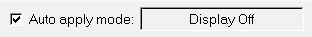
-
Go to the Contour panel
 .
.
- Select the first pull-down menu below Result type and select Element Stresses (2D & 3D).
- Select the second pull-down menu below Result type and select vonMises.
-
Above the Results Browser in the left hand panel are the
Load Case and Simulation Selection drop-down menus. Select Subcase 1
(Coup_Vert) from the Load Case drop-down menu.
Figure 5. 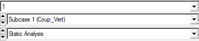
-
Click the XY Top Plane View icon
 to display a top view
of the Web.
to display a top view
of the Web.
-
Click Apply.
This should show the contour of stresses on the Web component under the coupled loading.
Figure 6. Stress Results on the Web From Nonlinear Gap Analysis 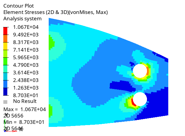
-
Click Delete Page
 to end the HyperView session.