Advanced Tube Element

Advanced Tube Description and Quick Guide

The advanced tube (AT) is a compressible flow element. It has many of the same inputs as the Incompressible Tube element but obviously the flow solution is different due to compressibility effects. The AT element could be used instead of the standard compressible tube element in models using a gas.

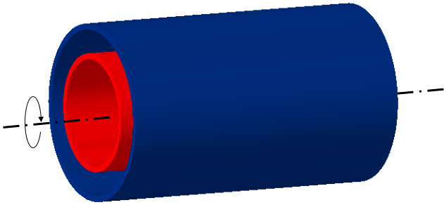
Some of the benefits of AT element over the standard compressible tube include the ability to divide the element walls into multiple circumferential segments and to use more than 20 axial segments. Each axial and circumferential segment of the AT can have unique friction and heat transfer inputs. The AT element can also calculate fluid swirl and windage changes for rotating annular passages or cylinders with the tube axis the same as the rotation axis.

The advanced tube element includes rotation (or gravity), wall friction, area change, and heat transfer effects. The advanced tube has a length and number of stations inputs like a standard tube. The wall friction and heat transfer effects use the length to determine the loss and temperature change. The losses due to sudden area change do not account for separated flow in this element. Use an expansion/contraction element to get losses when flow may separate due to the area change.

Flow in the advanced tube element is limited to subsonic. The maximum Mach number will be 1.0 and occur at the element exit station for a constant area duct. The maximum Mach number will occur at the minimum area for a duct with changing area. Use the Supersonic Tube element for converging-diverging geometries when the Mach number can exceed 1.

Advanced Tube Element Inputs

Table of the inputs for the advanced tube element.

Element Specific Input Variables

Index

UI Name (.flo label)

Description

Cross-Sectional Shape

(CS_SHAPE)

Specifies method for defining AT geometry parameters: hydraulic diameter (DHI), wetted perimeter (PWI), and flow area (AFI). The cross-section shape is also used to find an effective hydraulic diameter.

The following typical settings are set automatically by the GUI based on the selections made for Geometric Input Type and Size.

1: Circular AT with uniform area along the length of the AT. A single value for area is set in STATION_CS_AREAS

2: Circular AT with uniform diameter along the length of the AT. A single value for diameter is set in STATION_HYDDIAMS_OR_PERIMS

6: Arbitrary cross-sectional shape with uniform area and hydraulic diameter along the length of the AT. A single value for area is set on STATION_CS_AREAS and a single value for hydraulic diameter is set on STATION_HYDDIAMS_OR_PERIMS

7: Arbitrary cross-sectional shape with uniform area and wetted perimeter along the length of the AT. A single value for area is set on STATION_CS_AREAS and a single value for wetted perimeter is set on STATION_HYDDIAMS_OR_PERIMS

11: Tapered circular AT with area specified at inlet and exit. Assumes linear tapering of area. Inlet and exit area values are set on STATION_CS_AREAS

12: Tapered circular AT with diameter specified at inlet and exit. Assumes linear tapering of diameter. Inlet and exit diameter values are set on STATION_HYDDIAMS_OR_PERIMS

16: Tapered arbitrary cross-section shaped AT with area and hydraulic diameter specified at inlet and exit. Assumes linear tapering of area and hydraulic diameter. Inlet and exit area values are set on STATION_CS_AREAS. Inlet and exit hydraulic diameter values are set on STATION_HYDDIAMS_OR_PERIMS.

17: Tapered arbitrary cross-section shaped AT with area and wetted perimeter specified at inlet and exit. Assumes linear tapering of area and wetted perimeter. Inlet and exit area values are set on STATION_CS_AREAS. Inlet and exit wetted perimeter values are set on STATION_HYDDIAMS_OR_PERIMS.

21: Circular AT with area specified each station. Assumes linear tapering of area between stations. NUM_STATIONS number of area values are set on STATION_CS_AREAS

22: Circular AT with diameter specified each station. Assumes linear tapering of diameter between stations. NUM_STATIONS number of diameter values are set on STATION_HYDDIAMS_OR_PERIMS

26: Arbitrary cross-section shaped AT with area and hydraulic diameter specified each station. Assumes linear tapering of area and hydraulic diameter between stations. NUM_STATIONS number of area values are set on STATION_CS_AREAS. NUM_STATIONS number of hydraulic diameter values are set on STATION_HYDDIAMS_OR_PERIMS

27: Arbitrary cross-section shaped AT with area and wetted perimeter specified each station. Assumes linear tapering of area and wetted perimeter between stations. NUM_STATIONS number of area values are set on.

There are additional settings for triangle, rectangle, elliptical and annular shapes.

Number of Stations

(NUM_STATIONS)

Number of stations in the AT.

Station 1 is at the inlet plane; station NUM_STATIONS is at the exit plane. NSTA can range from 2 to unlimited. During the solution process, the AT will be discretized into NUM_STATIONS minus one segments with average temperatures, pressures, and Reynolds Numbers for each segment.

An advanced tube should be modelled with at least 2 stations. The number of stations can have a big impact on the convergence of attached chambers. If a chamber attached to this element is having difficulty converging, try increasing the number of stations. Of course, analysis speed may decrease as the number of stations increase.

Number of AT wall sides

(NUM_WALL_SIDES)

Number of circumferential wall segments around the AT. Wall segments can have their own loss mode, heat transfer mode, roughness definition, and turbulator definitions (heat transfer, friction, geometry).

Number of bends

(NUM_BENDS)

Number of bends in the AT. Each bend is defined by a bend radius, bend angle, location in the AT (either distance from start of AT, or a specified straight segment length between bends), loss multiplier and combination angle.

Total Length

(LENGTH)

Length of the AT in inches. Do not include length within bends unless the bend losses are not otherwise accounted.

Station Length Fraction

(STATION_MODE)

Flag specifying station location definitions.

0: Stations are uniformly distributed along the length of the AT

1: Station location is defined as a percentage of length of the AT. User specifies percentage for each station in the STATION_LOCATIONS array. Valid values are 0-100.

2: Station location is defined as distance from the start of the AT. User specifies distance from start for each station in the STATION_LOCATIONS array. Valid values are 0-LENGTH

Turbulent Friction Relation

(FRIC_RELATION)

A flag that specifies which friction relation is used.

0.0: Smooth Wall Power law (Abuaf)

1.0: Swamee-Jain (approx. to Colebrook-White)

Swamee-Jain (1.0) is recommended for non-zero roughness.

Roughness type

(ROUGH_TYPE)

Flag specifying measurement method of user-input ROUGHNESS value. Roughness values will be converted to sand-grain roughness equivalent. For more information see Friction Correlations section in General Functions and Routines.

0: Equivalent sand-grain roughness

1: Average absolute roughness

2: Root mean square roughness

3: Peak-to-valley roughness

HTC Relation

(HTC_RELATION)

The “Duct Flow” Nu correlation used for turbulent flow.

See the “HTC Correlations” in the “General Functions and Routines” section for the equations.

-2) User Input Nu

-1) User Input HTC

1) Lapides-Goldstein

2) Dittus-Boelter

3) Sieder-Tate Combo

4) Gnielinski Combo

5) Bhatti-Shah

7) Sieder-Tate Turbulent Only

8) Gnielinski-Turbulent Only

9) Rotating Parallel Duct (Morris)

41) Rotating Shaft (Seghir-Ouali and Gai)

Heat Transfer Inlet Effects

(HT_INLET_EFF)

Flag specifying heat transfer inlet effects applied for the AT.

See the Heat Transfer Coefficients (HTC) section in General Functions and Routines.

0: No inlet effects

1: Abrupt local or uniform average inlet effects

3: Abrupt average inlet effects

4: Uniform local inlet effects

5: Between uniform average and local inlet effects

6: Between abrupt average and local inlet effects

Portion of Ustrm Cham. Dyn. Head Lost

(DQ_IN)

Inlet dynamic head loss. Valid range is 0.0 to 1.0 inclusive. An entry outside this range will cause a warning message and the value used will be 0 or 1 (whichever value is closest to the entry).

If DQ_IN > 0 and the upstream chamber has a positive component of relative velocity aligned with the centerline of the tube, the driving pressure will be reduced by the equation:

$P i n = P s_{u p s t r e a m} + (1.0 - D Q_{I N}) * (P i n_{n o - l o s s} - P s_{u p s t r e a m})$

(Default value = 0.)

Rotor Index

(RPMSEL)

Element rotational speed pointer.

-1: Rotates with air.

0.0: Specifies a stationary element.

1.0: Rotor 1, RPM = general data ELERPM(1).

2.0: Rotor 2, RPM = general data ELERPM(2).

3.0: Rotor 3, RPM = general data ELERPM(3).

Gravity Multiplier

(GRAV_MULT)

Multiplier on the constant for acceleration due to gravity, G_c. G_c is nominally equal to 32.17405 lbm-ft/lbt-sec². Gravity effects only available when AT is stationary.

Element Inlet Orientation: Tangential Angle

(THETA)

Angle (deg) between the element centerline at the entrance of the element and the reference direction.

If the element is rotating or directly connected to one or more rotating elements, the reference direction is defined as parallel to the engine centerline and the angle is the projected angle in the tangential direction. Otherwise, the reference direction is arbitrary but assumed to be the same as the reference direction for all other elements attached to the upstream chamber.

Theta for an element downstream of a plenum chamber has no impact on the solution except to set the default value of THETA_EX.

(See also THETA_EX)

Element Inlet Orientation: Radial Angle

(PHI)

Angle (deg) between the element centerline at the entrance of the element and the THETA direction. (spherical coordinate system)

Phi for an element downstream of a plenum chamber has no impact on the solution except to set the default value of PHI_EX.

(See also PHI_EX)

Exit K Loss:

Axial (K_EXIT_Z)

Tangential (K_EXIT_U)

Radial (K_EXIT_R)

Head loss factors in the Z, U, and R directions based on the spherical coordinate system of theta and phi.

Z = the axial direction. (theta=0 and phi=0)

U = the tangential direction. (theta=90 and phi=0)

R = the radial direction. (theta=0 and phi=90)

Valid values of K_EXIT_i (i = Z, U, R) range from zero (default) to one.

The three loss factors reduce the corresponding three components of velocity exiting the element.

$V_{a c t u a l e x i t i d i r} = V_{n o l o s s e x i t i d i r} * \sqrt{1 - K_E X I T_i d i r}$

(Default value provides no loss, K_EXIT_i=0)

Element Exit Orientation: Tangential Angle

(THETA_EX)

Angle (deg) between the element exit centerline and the reference direction.

THETA_EX is an optional variable to be used if the orientation of the element exit differs from that of the element inlet.

The default value (THETA_EX = -999) will result in the assumption that THETA_EX = THETA.

Other values will be interpreted in the manner presented in the description of THETA.

Element Exit Orientation: Radial Angle

(PHI_EX)

Angle (deg) between the element exit centerline and the THETA_EX direction.

PHI_EX is an optional variable to be used if the orientation of the element exit differs from that of the element inlet.

The default value (PHI_EX = -999) will result in the assumption that PHI_EX = PHI.

Other values will be interpreted in the manner presented in the description of PHI.

Nusselt Number for Laminar Flow

(NU_LAM)

Nusselt number used in the laminar flow region (defaults to 4.36)

(RE_POW)

Not Used

(MDOT_REF)

Not Used

Pressure Tolerance Value

(PRESSURE_TOL)

User defined inlet total pressure convergence tolerance.

Caution should be used when increasing this very much above the default value.

The total pressure calculated from the station marching from exit to inlet must match the total pressure of the upstream chamber minus any losses (PTIN)

Defaults to 0.000001 psia.

Mach Number Tolerance Value

(MACH_TOL)

User defined convergence tolerance for a station mass flows. Mass flow continuity is achieved by changing station Mach numbers until convergence criteria is met.

Defaults to 0.000001 lbm/sec

Aspect Ratio

(ASPECT_RATIO)

The aspect ratio of the AT cross section for an Arbitrary-Shape cross section. The aspect ratio should be between 0 and 1.

Laminar Friction Effects

(LAMR_FRIC_RLTN)

Laminar friction effects to use at the duct inlet. See the “Friction Correlations” in the “General Functions and Routines” section for the equations.

0) Off, assume fully developed laminar flow.

1) Muzychka-Yovanovich

Laminar HTC Relation

(NU_LAM_METHOD)

The “Duct Flow” Nu correlation used for laminar flow.

See the “HTC Correlations” in the “General Functions and Routines” section for the equations.

0) User Input Nu

1,4,5) Muzychka-Yovanovich

2) Hausen

No GUI Input

(PROPS_METHOD)

Temperature to be used for fluid properties retrieval.

Properties at the local temperature (default)
Properties at average bulk fluid temperature (T_inlet+T_outlet)/2

Inner Diameter (ID) Rotor Index

(RPMSEL_INNER)

The rotation of the inner diameter wall of an annulus.

Used only for ROTATION_METH=1, Rotating Annulus.

0.0: Specifies a stationary inner annulus wall.

1.0: Rotor 1, RPM = general data ELERPM(1).

2.0: Rotor 2, RPM = general data ELERPM(2).

3.0: Rotor 3, RPM = general data ELERPM(3).

Inlet Head Loss Type

(K_IN_METHOD)

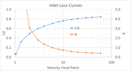
The type of inlet losses.

K – Incompr Loss Coef

K_in = inlet head loss / dynamic head,

or $K_{i n} = \frac{P_{T, s u p p l y} - P_{T, a f t e r l o s s}}{0.5 ρ V^{2}}$

1) Cd – Compr Loss Coef

$K_{i n} = {(\frac{1.0}{C d})}^{2} - 1.0$

2) Upstream Cross Flow

The inlet loss is assumed to be due to a cross flow velocity at the inlet and is calculated according to Ref. 3.

The data used is for a tube with L/D > 2.83, where the flow has recovered from the inlet effects and is at right angles to the cross flow.

The method is valid for both upstream momentum and upstream inertial chambers. It is not valid for upstream plenum chambers.

33-35

(FUTURE)

Reserved for future development

Bend Input Mode

(BEND_INPUT_MODE)

Flag indicating how the locations of bends are defined.

0: Bend location is distance from start of the AT in inches.

1: Bend location is defined by the distance of straight AT length between the end of the previous bend (or inlet, if it is the first bend) and the beginning of the current bend

Laminar-to-Transition Reynolds Number

(RE_LAM)

Reynolds number below which flow is assumed to be laminar

Transition-to-Turbulent Reynolds Number

(RE_TURB)

Reynolds number above which flow is assumed to be turbulent. Flow at Reynolds numbers between RE_LAM and RE_TURB are assumed to be in the transition region.

Friction Type

(FRIC_TYPE)

Friction factor output type.

1: Darcy friction factor

2: Fanning friction factor

Starting Length

(STLEN)

Starting length (in) used for the HTC inlet multiplier.

Used to modify X in calculating h_x/h_o:

$X = X_{m e a s} + S T L E N$

where X_meas = Distance from AT inlet (station 1).

At station 1, X equals STLEN. If one physical AT is modelled as two or more elements strung together, STLEN should include the cumulative length of all AT elements leading into the current element unless something physical re-establishes the boundary layer.

Inlet Head Loss

(K_INLET)

Inlet head loss.

This is either a K or Cd depending on K_IN_METHOD.

42-45

(FUTURE)

Reserved for future development

Rotation Method

(ROTATION_METH)

Method for applying element rotation effects. Option 0 is the traditional method where all element walls are rotating at the same speed and the fluid is rotating at same speed as the walls. Options 1 and 2 calculate swirl and windage change along the length of the tube.

0: Stationary or Forced to Rotor Speed

1: Rotating Annulus

2: Rotating Coaxial Shaft

Bend Radius

(BEND_RADIUS)

(array of 20 values in 4 lines of 5 each, NUM_BENDS values used)

Radius (in) of bend along AT centerline.

(See ‘ r ’ from graphic for COMBINATION_ANGLE below)

Each bend counted in NUM_BENDS must have a specified bend radius. Enter bends in order based on distance from beginning of AT (DIST_FR_STRT).

Bend Angle

(BEND_ANGLE)

(array of 20 values in 4 lines of 5 each, NUM_BENDS values used)

Angle (deg) between the entering and exiting lengths of the bend.

Each bend must have a specified angle.

The maximum bend angle is 180°.

Distance from Start

(DISTANCE)

(array of 20 values in 4 lines of 5 each, NUM_BENDS values used)

Array of values that indicate bend location in the AT. The interpretation of the values in the array depends on the value of BEND_INPUT_MODE:

BEND_INPUT_MODE = 0: DISTANCE is cumulative straight AT segment length (in.) to the start of the current bend,

BEND_INPUT_MODE = 1: DISTANCE is straight segment length (in.) from end of the previous bend (or inlet if it is the first bend in the AT) to the start of the current bend.

Loss Multiplier

(LOSS_MULT)

(array of 20 values in 4 lines of 5 each, NUM_BENDS values used)

Loss multiplier for each bend (Default = 1.0).

Combination Angle

(COMBINATION_ANGLE)

(array of 20 values in 4 lines of 5 each, NUM_BENDS minus one values used)

Relative angle (deg) between two bends in series.

The number of COMBINATION_ANGLE entries will be NUM_BENDS – 1. The first entry will be the combination angle between bends 1 and 2.

A COMBINATION_ANGLE of 0 degrees defines an ‘S’ shaped bend and 180 degrees defines a ‘U’ shaped bend.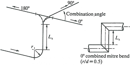

Figure 2. Notation for combination of two 90° bends (Ref 5, pg. 228)

The allowable range is 0 to 180 degrees.

STATION_LOCATIONS

(Dynamic array of NUM_STATIONS values)

Dynamic array of NUM_STATIONS station locations, specified as a percentage of length, a fraction of length, or a distance from start of AT, depending on the value of STATION_MODE. For STATION_MODE = 0 (uniformly distributed), this array will not be used.

STATION_RADII

(Dynamic array of NUM_STATIONS values)

Dynamic array of NUM_STATIONS station radii in inches. Only applicable for rotating ATs, that is, RPMSEL not equal to 0.

STATION_HEIGHTS

(Dynamic array of NUM_STATIONS values)

Dynamic array of NUM_STATIONS station heights in inches. Only applicable for stationary ATs, that is, RPMSEL = 0, and when gravitational effects are enabled. Station height is defined as distance above a datum and is used to determine gravitational effects on the fluid.

Station cross-section areas

(STATION_CS_AREAS, dynamic array, length depends on value of CS_SHAPE)

Dynamic array of station cross-section areas. Length of the array is determined by the value of CS_SHAPE. STATION_CS_AREAS is only used for CS_SHAPE = 1, 6, 7, 11, 16, 17, 21, 26, or 27


CS_SHAPE	Description	Form of CS_AREAS
1	Circular AT with uniform area	1 value = AT area
6	Arbitrary cross-section AT with uniform area and hydraulic diameter	1 value = AT area
7	Arbitrary cross-section AT with uniform area and wetted perimeter	1 value = AT area
11	Tapered circular AT with area specified at inlet and exit	2 values = inlet and exit area
16	Tapered arbitrary cross-section shaped AT with area and hydraulic diameter specified at inlet and exit	2 values = inlet and exit area
17	Tapered arbitrary cross-section shaped AT with area and wetted perimeter specified at inlet and exit	2 values = inlet and exit area
21	Circular AT with area specified at each station	NUM_STATIONS values = station area
26	Arbitrary cross-section shaped AT with area and hydraulic diameter specified at each station	NUM_STATIONS values = station area
27	Arbitrary cross-section shaped AT with area and wetted perimeter specified at each station	NUM_STATIONS values = station area

A10

Station hydraulic diameter or wetted perimeter

(STATION_HYDDIAMS_OR_PERIMS, dynamic array, length and meaning of value depends on value of CS_SHAPE)

Dynamic array of station hydraulic diameter or perimeter. Length of and meaning of value in the array is determined by the value of CS_SHAPE. STATION_HYDDIAMS_OR_PERIMS is only used for CS_SHAPE = 2, 6, 7, 12, 16, 17, 22, 26, or 27


CS_ SHAPE	Description	Form of CS_HYDIAMS_ OR_PERIMS
1	Circular AT with uniform area	1 value = 0
2	Circular AT with uniform diameter	1 value = D_h
6	Arbitrary cross-section AT with uniform area and hydraulic diameter	1 value = = D_h
7	Arbitrary cross-section AT with uniform area and wetted perimeter	1 value = P_w
11	Tapered circular AT with area specified at inlet and exit	1 values = 0
12	Tapered circular AT with diameter specified at inlet and exit	2 values = D_in, D_exit
16	Tapered arbitrary cross-section shaped AT with area and hydraulic diameter specified at inlet and exit	2 values = D_h,in,D_h,exit
17	Tapered arbitrary cross-section shaped AT with area and wetted perimeter specified at inlet and exit	2 values = P_w,in,P_w,exit
21	Circular AT with area specified at each station	1 value = 0
22	Circular AT with diameter specified at each station	NUM_STATIONS values = D_h,station
26	Arbitrary cross-section shaped AT with area and hydraulic diameter specified at each station	NUM_STATIONS values = D_h,station
27	Arbitrary cross-section shaped AT with area and wetted perimeter specified at each station	NUM_STATIONS values = P_w,station

A11

WALL_SIDE_FRACTIONS

(Dynamic array of length NUM_WALL_SIDES)

Array of length NUM_WALL_SIDES specifying the portion of the AT perimeter represented by each wall side (segment). WALL_SIDE_FRACTIONS can be input as either a fraction or a percentage. If input as a fraction:

$\sum_{i = 1}^{N U M_W A L L_S I D E S} W A L L_S I D E_F R A C T I O N S (i) = 1.0$

And if input as a percentage:

$\sum_{i = 1}^{N U M_W A L L_S I D E S} W A L L_S I D E_F R A C T I O N S (i) = 100 %$

Wall sides cover the length of the AT and thus apply at every station.

A12

WALL_SIDE_TYPES

(Dynamic array of length NUM_WALL_SIDES)

Array of length NUM_WALL_SIDES specifying the surface type of each wall side (segment).

0: Smooth surface

1: Rough surface

2: Turbulated surface

For types 1 and 2, additional inputs are required to define roughness and/or turbulator geometry.

Wall sides cover the length of the AT and thus apply at every station.

A13

LOSS_MODE_ON_EACH_SIDE

(Dynamic array of length NUM_WALL_SIDES)

Array of length NUM_WALL_SIDES specifying the momentum loss calculation method for each wall side (segment).

0: No momentum loss

1: Specified roughness, uniform along AT length

2: Specified friction coefficient, uniform along AT length

3: Specified K_loss, uniform along AT length

4: Specified friction multiplier applied to calculated friction, uniform along AT length

12: Linearly tapered friction coefficient, specified at inlet and exit

14: Linearly tapered friction multiplier applied to calculated friction, specified at inlet and exit

21: Specified roughness for each AT segment (between stations)

22: Specified friction coefficient for each AT segment (between stations)

23: Specified K_loss for each AT segment (between stations)

24: Specified friction multiplier applied to calculated friction for each AT segment (between stations)

The choice of LOSS_MODE_ON_EACH_SIDE will determine the length of and interpretation of the values in the LOSS_QUANTITIES_ON_SIDE_X arrays

Wall sides cover the length of the AT and thus apply at every station.

A14

HEAT_MODE_ON_EACH_SIDE

(Dynamic array of length NUM_WALL_SIDES)

Array of length NUM_WALL_SIDES specifying the heat transfer calculation method for each wall side (segment).

0: Adiabatic

1: Uniform heat load (Btu/s)

2: Uniform heat load (Btu/lbm)

3: Uniformly distributed delta T (Not implemented)

4: Fixed fluid total temperature at AT exit (Not implemented)

5: Calculated inner wall convection

6: Inner wall convection with constant Nusselt number

7: Inner wall convection with constant heat transfer coefficient

8: Calculated inner wall convection with constant Hmult

16: Inner wall convection with linearly tapered Nusselt number, specified at inlet and exit.

17: Inner wall convection with linearly tapered HTC, specified at inlet and exit.

18: Calculated inner wall convection with linearly tapered Hmult, specified at inlet and exit.

21: Specified heat load (Btu/s) at each AT segment (between stations)

22: Specified heat load (Btu/lbm) at each AT segment (between stations)

23: Specified delta T across each AT segment (between stations) (Not implemented)

24: Specified total temperature at each AT station (Not implemented)

26: Inner wall convection with Nusselt number specified for each AT segment (between stations)

27: Inner wall convection with HTC specified for each AT segment (between stations)

28: Calculated inner wall convection with Hmult specified for each AT segment (between stations)

The choice of HEAT_MODE_ON_EACH_SIDE will determine the length of and interpretation of the values in the HEAT_QUANTITIES_ON_SIDE_X arrays

Wall sides cover the length of the AT and thus apply at every station.

A15

LOSS_QUANTITIES_ON_SIDE_X

These arrays hold the loss quantities on side number X. There will be NUM_SIDES number of these arrays in the database and their length and interpretation of contained values is determined by the value of LOSS_MODE_ON_EACH_SIDE as follows:


LOSS_ MODE_ON_ EACH_SIDE	Description	Form of LOSS_QUANTITIES_ON_SIDE_X
0	No momentum loss	1 value = 0 (not used)
1	Specified uniform roughness	1 value = roughness
2	Specified uniform friction coefficient	1 value = friction coefficient
3	Specified uniform K_loss	1 value = K_loss
4	Specified uniform friction multiplier	1 value = friction multiplier
12	Linearly tapered friction coefficient, specified at inlet and exit	1 value = friction coefficient
14	Linearly tapered friction multiplier, specified at inlet and exit	1 value = friction multiplier
21	Specified roughness for each AT segment (between stations)	(NUM_STATIONS – 1) values = segment roughness
22	Specified friction coefficient for each AT segment (between stations)	(NUM_STATIONS – 1) values = segment friction coefficient
23	Specified K_loss for each AT segment (between stations)	(NUM_STATIONS – 1) values = segment K_loss
24	Specified friction multiplier for each AT segment (between stations)	(NUM_STATIONS – 1) values = segment friction multiplier

NOTE: Interpretation of roughness values specified for LOSS_QUANTITIES_ON_SIDE_X will depend on the value of the ROUGH_TYPE input parameter.

A15

HEAT_QUANTITIES_ON_SIDE_X

These arrays hold the heat transfer quantities on side number X. There will be NUM_SIDES number of these arrays in the database and their length and interpretation of contained values is determined by the value of LOSS_MODE_ON_EACH_SIDE as follows:


HEAT_ MODE_ON_ SIDE_X	Description	Form of LOSS_QUANTITIES_ON_SIDE_X
0	Adiabatic	1 value = 0 (not used)
1	Uniform heat load (BTU/s)	1 value = Heat load in BTU/s
2	Uniform heat load (BTU/lbm)	1 value = Heat load in BTU/lbm
3	Uniformly distributed ΔT	1 value = ΔT across the whole AT in ^oF
4	Fixed fluid total temperature at AT exit	1 value = TT_exit (^oF)
5	Calculated inner wall convection	1 value = 0 (not used)
6	Inner wall convection with constant Nusselt number	1 value = Nu
7	Inner wall convection with constant HTC number	1 value = HTC (Btu/hr-ft²-^oF)
8	Calculated inner wall convection with constant Hmult	1 value = Hmult
16	Inner wall convection with linearly tapered Nusselt no.	2 values = Nu_in, Nu_exit
17	Inner wall convection with linearly tapered HTC	2 values = HTC_in, HTC_exit
18	Calculated inner wall convection with linearly tapered Hmult	2 values = Hmult_in, Hmult_out
21	Specified heat load (BTU/s) at each AT segment (between segments)	(NUM_STATIONS – 1) values = heat load (BTU/s)
22	Specified heat load (BTU/lbm) at each AT segment (between segments)	(NUM_STATIONS – 1) values = heat load (BTU/lbm)

A15

HEAT_QUANTITIES_ON_SIDE_X

(Continued)


HEAT_ MODE_ON_ SIDE_X	Description	Form of LOSS_QUANTITIES_ON_SIDE_X
23	Specified ΔT across each AT segment (between stations)	(NUM_STATIONS – 1) values = ΔT_segment (^oF)
24	Specified fluid total temperature at each station	NUM_STATIONS values = TT_station
26	Inner wall convection with Nusselt number specified for each segment (between stations)	(NUM_STATIONS – 1) values = Nu_segment
27	Inner wall convection with HTC specified for each AT segment (between stations)	(NUM_STATIONS – 1) values = HTC_segment
28	Calculated inner wall convection with Hmult specified for each AT segment (between stations)	(NUM_STATIONS – 1) values = Hmult_segment

NOTE: For Heat Modes using calculated inner wall convection, the method of heat transfer calculation is determined by the value of the HTC_RELATION input parameter.

A16

WALL_TEMPERATURE_ON_SIDE_X

(Dynamic array, number of values is input by the user)

Surface temperature of the AT wall for use in heat transfer and fluid calculations. The user has three options for number of values to input for wall temperature. The size of the array determines how the values in the array are determined:


Size of Array	Interpretation of Values
1 Value	Uniform wall temperature (^oF) along the whole AT
2 Values	Inlet and exit wall temperature (^oF) linearly interpolated along the length of the AT
NUM_STATIONS Values	Wall temperature (^oF) specified at every station along the AT

Advanced Tube Element Theory Manual

The advanced tube element routine simulates compressible gas flow through a passage where friction is a significant pressure loss mechanism. Both laminar and turbulent flows are accommodated by the routine as is heat transfer with either internal turbulators or with conduction/convection/radiation using thermal networks.

The length of the AT is divided into segments of arbitrary length, the number of segments, typically (but not limited to) between 5 and 15, being that specified in the input file. The beginning and end of each segment is represented as a “station” so there is one more station than the number of segments used for the AT. The geometry of the AT flow passage is defined by a combination of two of the three input variables, flow area, hydraulic diameter, and wetted perimeter, specified for each of the AT stations, the remaining variable being calculated using the equation:

D_{h y d} = \frac{4 * A r e a}{P e r i m e t e r}

The AT routine is divided into two main sections: a flow direction calculation and a flow iteration loop. In the flow direction section, the procedures described in the paragraphs on computing the element flow inlet and outlet conditions are employed to define the inlet driving pressure (PTS), the inlet temperature, the secondary fluid mass fraction, and the exit back pressure (PSEB). If the AT is rotating and its inlet and outlet are at different radii, an estimate of the pumping effect due to rotation is used to compute an effective inlet pressure, PTSM. The procedure used to calculate the pressure ratio, PTSM / PTS, is identical to that for a forced vortex turning at the specified element RPM. If PTS (or PTSM) is greater than PSEB, these pressures are employed with a simple overall flow coefficient, based on inlet pressure drop and estimated friction effect, to estimate the fluid velocity at the AT exit plane. If PTS (or PTSM) is less than PSEB,, the calculation is repeated with the flow direction reversed.

The mass, momentum, and energy conservation must be maintained along the length of the AT. The conservation equations solved in the advanced tube are the same as those solved for the compressible tube although the solution method is different. The equations and methods used are described here.

Mass Equation

The continuity equation is given as:

\dot{m} = ρ A v = c o n s t a n t f o r e a c h t u b e s t a t i o n

Momentum Equation

The momentum equation is given as (ref 2):

\int ρ A V d V = \int - A d p + \int d F_{f} + \int d F_{b}

Where:

d F_{f} = f r i c t i o n a l f o r c e s = \frac{f ρ V^{2}}{2 D_{h}} d x

d F_{b} = c e n t r i f u g a l f o r c e s = A \frac{ρ ω^{2}}{r} d x

Combined Equation

The mass and momentum equations can be combined to give (ref 2):

\int_{M_{x}}^{M_{x + Δ x}} \frac{(1 - M^{2})}{M (1 + \frac{γ - 1}{2} M^{2})} d M = \int_{x}^{x + Δ x} [\frac{γ M^{2} f}{2 D_{h}}] d x + \int_{x}^{x + Δ x} [\frac{1 + γ M^{2}}{2}] \frac{d T_{T}}{T_{T}} - \int_{x}^{x + Δ x} [\frac{ω^{2}}{2 R T_{s}}] d (r^{2}) = I_{m}

The total pressure ratio across a segment can be related to the integral ( $^{I_{m}}$ ) by:

\frac{P_{t x + Δ x}}{P_{t}} = e^{I_{m}}

Inlet Head Loss

Having calculated (or guessed) a Mach number just inside the element inlet, inlet head loss computations are made to determine the total pressure, $P t_{i}$ , at this location. The simplest loss function is a constant K-loss input value (K) that is used in the following equation to calculate $P t_{i}$ :

P t_{i} = \frac{P t_{s}}{1 + K * q / P t_{i}}

q = d y n a m i c p r e s s u r e = \frac{1}{2} * ρ * V^{2}

P t_{s} = u p s t r e a m s o u r c e p r e s s u r e (b e f o r e K l o s s)

There is also an option to calculate an inlet K loss based on a built-in correlation based on data reported in Ref 3, Fig 8. Converting Cd from the plot to head loss using:

K_{i n} = {(\frac{1.0}{C d})}^{2} - 1.0

V e l H e a d R a t i o = \frac{(P t_{s} - P s_{t u b e_i n l e t})}{(P t_{s} - P s_{u p s t r e a m c h a m b e r})}

In addition to the inlet losses, pressure losses due to bends can also be included in the AT element. There are 2 ways to model bend losses in Flow Simulator: 1) include the bend in the AT element, 2) Use a separate bend element with the AT element only accounting for the straight length. Each method has advantages and disadvantages. Option 2 may lead to more accurate results and allows for the pressures upstream and downstream of the bends to be visible in the GUI. Option 1 is faster, and accuracy is sufficient for engineering calculations. If option 1 is used, the bend K loss is calculated the same way as the bend element K loss (see the bend element for calculation details).

Energy Equation

Start with the differential form of the steady state energy balance equation:

\frac{d H}{d x} = \dot{m} C_{p} \frac{d T}{d x} = h C (T_{w} - T) + \dot{m} (ω^{2} r \frac{d r}{d x} - g_{c} \frac{d z}{d x}) + q_{i n}^{'} (x)

The AT uses the following energy integral [ref 4 section 1.6]:

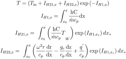
These integrals are calculated in a semi-analytic way.

Integral $I_{H 1, x}$ is calculated as:

Integral $I_{H 21, x}$ is calculated as:

Where:

Integral $I_{H 22, x}$ is calculated as:

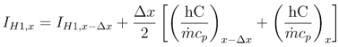
Finally, temperature at location x is calculated as:

Coupling with the Thermal Network Solver

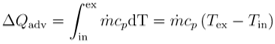
The total amount of heat added to the fluid is given by:

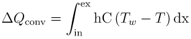
Heat added, $Δ Q_{a d v}$ , is a result of convection from the AT wall:

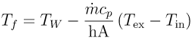
Wall temperature along a segment is constant and we assume that there is a fluid temperature that satisfies:

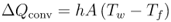
The fluid temperature can be calculated as:

Rotating Annulus and Coaxial Shaft Angular Momentum Balance

If the rotation method is “Rotating Annulus” or “Rotating Coaxial Shaft”, an angular momentum balance equation is solved to calculate the change of fluid swirl and fluid temperature due to windage. These rotation methods require that the element is attached to inertial chambers at each end. These rotation methods can be used instead of cavities for long annular or coaxial cylinders. For example, the Rotating Annulus method is used between the red and blue cylinders while the Rotating Coaxial Shaft is used inside the red cylinder in this figure.

The angular momentum equation that is solved:

T q_{r} - T q_{s} = \dot{m} * ω * (R_{o u t} * X K_{o u t} - R_{i n} * X K_{i n})

T q_{r} = t o r q u e f r o m t h e r o t o r s u r f a c e

T q_{s} = t o r q u e f r o m t h e s t a t o r s u r f a c e

\dot{m} = m a s s f l o w r a t e t h r o u g h t h e t u b e

ω = r o t a t i o n a l s p e e d (r a d / s)

\begin{array}{l} X K_{i n, o u t} = R a t i o o f t h e f l u i d a b s o l u t e r o t a t i o n a l s p e e d t o t h e r o t a t i o n a l \\ r e f e r e n c e f r a m e a t i n l e t a n d e x i t o f t h e t u b e s e g m e n t \end{array}

R_{i n, o u t} = F l o w r a d i u s a t i n l e t a n d e x i t o f t h e t u b e s e g m e n t

The flow radius is always the center of an annulus, but the flow radius is not well defined for a Rotating Coaxial Shaft. You must supply the flow radius for the Rotating Coaxial Shaft method. If the flow radius is 0, the XK=1 and the fluid is rotating at the same speed as the shaft. A flow radius of 0.25 times the shaft diameter is a good value to use unless experience indicates a different value.

The torque equations use the same skin friction coefficient equations used for cylindrical surfaces in cavities.

The Reynolds number will use an effective velocity based on axial and rotational velocities. This effective Reynolds number is used in the heat transfer coefficient and friction calculations. Furthermore, the friction uses an effective length to account for the spiral path of the flow through the tube. See reference 6 by Gazley.

V_{e f f} = \sqrt{V_{a x i a l}^{2} + V_{r e l a t i v e_t a n g e n t i a l}^{2}}

R e_{e f f} = \frac{ρ V_{e f f} D_{h}}{μ}

A table of results is written to the .res file for these rotation methods. This table contains swirls, relative tangential velocities, and torques at each tube station.

Solution Method

The main steps in the solution method are:

Guess an exit station Mach number.
Calculate an exit station flowrate using the exit station Mach number.
Loop through each AT station from the exit to the inlet.
- Calculate a station temperature, Mach number, and pressure that satisfies the mass, momentum, and energy equations.
Compare the inlet station total pressure with the total pressure of the upstream chamber minus any losses (PTI).
If the inlet total pressures do not match within the convergence tolerance, adjust the exit station Mach number, and repeat steps 2-4.

Advanced Tube Element Outputs

The following listing provides details about the elements output variables.


Name	Description	Units
CROSS-SECTION	Shape of AT cross-section.	(None)
LENGTH	Length of the AT.	Inch, m
NUM_STATIONS	Number of stations in the AT.	(None)
NUM_CIRCUMF_WALL_SEGS	Number of circumferential wall segments around the AT.	(None)
RI	AT inlet radius.	Inch, m
RE	AT exit radius.	Inch, m
K_INLET	Inlet head loss (user input).	(None)
FRICTION_TYPE	Friction factor calculation used in the solution (DARCY, FANNING, or N/A).	(None)
TURB_FRIC	Turbulent friction relation used for solution (ABAUF (Smooth Wall Power Law), SWAMEE (Colebrook White), or OFF).	(None)
LAM_FRIC	Laminar friction relation used for the solution.	(None)
INPUT_ROUGHNESS_ TYPE	Roughness input type used for solution (SAND_GRAIN, AVERAGE_ABSOLUTE, ROOT_MEAN_SQUARE, or PEAK_TO_VALLEY).	(None)
K_CONTRAC_RESULT	Back-calculated K loss.	(unitless)
CD_RESULT	Result calculated from actual mass flow rate divided by ideal mass flow rate. The ideal mass flow rate assumes K=0.	(unitless)
QTOTAL	Total heat change over the entire AT.	Btu/s, W
PTS	Driving pressure relative to the rotational reference frame (that is, rotor) at the AT inlet.	psia, MPa
PTIN	Total pressure relative to the rotational reference frame (that is, rotor) at the AT inlet, includes inlet losses.	psia, MPa
PSIN	Static pressure relative to the rotational reference frame (that is, rotor) at the AT inlet. Limited by critical pressure ratio for supersonic flows when inlet area is smaller than exit area.	psia, MPa
PTEX	Total pressure relative to the rotational reference frame (that is, rotor) at the AT exit including supersonic effects.	psia, MPa
PSEX	Static pressure relative to the rotational reference frame (that is, rotor) at the AT exit. Limited by critical pressure ratio for supersonic flows.	psia, MPa
PSEB	Effective sink (static) pressure downstream of the AT.	psia, MPa
TTS	Total temperature of fluid relative to the rotational reference frame (that is, rotor) at the AT inlet.	degF, K
TSIN	Static temperature of fluid relative to the rotational reference frame (that is, rotor) at the AT inlet.	degF, K
INVEL	Velocity of fluid relative to the rotational reference frame (that is, rotor) at the transition inlet.	ft/s, m/s
TTEX	Total temperature of fluid relative to the rotational reference frame (that is, rotor) at the AT exit.	degF, K
TSEX	Static temperature of fluid relative to the rotational reference frame (that is, rotor) at the AT exit.	degF, K
EXVEL	Velocity of fluid relative to the rotational reference frame (that is, rotor) at the transition exit.	ft/s, m/s
Station Geometry	Table of AT geometry.	NONE
STA	Column of stations. Station 1 is listed as “Inlet” and station NUM_STATIONS is listed as “Exit”.	NONE
X	Station location as a distance from the inlet.	Inch, m
RADIUS	Station radius from engine center line.	Inch, m
HEIGHT	Station height from some datum, used in gravitational effects calculations.	Inch, m
DH	Station hydraulic diameter. If not user input, calculated from relation: Dh = 4*A/P.	Inch, m
PERIM	Station wetted perimeter. If not user input, calculated from relation: P = 4*A/Dh.	Inch, m
AREA	Station cross-sectional area. If not user input, calculated from relation: A=Dh*P/4.	in², m²
Station Bulk Data	Station-by-station fluid information.	NONE
PT	Fluid total pressure at station location.	psia, MPa
PS	Fluid static pressure at station location.	psia, MPa
TT	Fluid total temperature at station location.	degF, K
TS	Fluid static temperature at station location.	degF, K
VEL	Fluid velocity at station location.	ft/s, m/s
THETA	Fluid theta angle at station location. Will only change if there is a bend in the AT, otherwise it is the same as at “Inlet”.	deg
PHI	Fluid phi angle at station location. Will only change if there is a bend in the AT, otherwise it is the same as at “Inlet”.	deg
REYF	Fluid Reynolds number used in the friction calculation at the AT station. $R e_{y f} = \frac{\dot{m} D_{h}}{A μ_{f i l m}}$ $\dot{m} = t u b e m a s s f l o w$ $D_{h} = t u b e h y d r a l i c d i a m e t e r$ $A = t u b e a r e a$ $μ_{f i l m} = f l u i d v i s c o s i t y b a s e d o n T_{f i l m}$ $T_{f i l m} = \frac{T_{s} + T_{w a l l}}{2}$	Unitless
REGIME	Flow regime at current station (TURB, LAM, or TRAN).	NONE
RHO	Fluid density at station location.	lbm/ft³, kg/m³
CP	Fluid specific heat at station location.	Btu/lbm-^oF, J/kg-^oK
Segment Bulk Data	Segment-by-segment heat addition/temperature rise results.
KSEG	Head loss (K-loss) across the current segment.	NONE
Q_CONV	Heat added to fluid across segment due to convection.	Btu/s, W
Q_FLUX	Heat added to fluid across segment due to heat flux.	Btu/s, W
Q_ROTA	Heat added to fluid across segment due pumping.	Btu/s, W
Q_GRAV	Heat added to fluid across segment due to buoyancy (gravitational effects).	Btu/s, W
Q_TOT	Total heat added to fluid across segment.	Btu/s, W
DTCONV	Fluid temperature rise (or fall) across segment due to convection.	degF, K
DTFLUX	Fluid temperature rise (or fall) across segment due to heat flux.	degF, K
DTROTA	Fluid temperature rise (or fall) across segment due to pumping.	degF, K
DTGRAV	Fluid temperature rise (or fall) across segment due to buoyancy (gravitational effects).	degF, K
DTTOT	Total fluid temperature rise (or fall) across segment.	degF, K
Station Data for Circumferential Wall Segment X	Station-by-station data for each circumferential wall segment in the model.	NONE
WFRAC	Fraction of the AT circumference modeled by the current wall side segment.	NONE
ARC	Arc length of AT modeled by the current wall side segment.	Inch, m
TWALL	User defined wall temperature.	degF, K
TFILM	Fluid temperature used to determine fluid properties for heat transfer calculations (Cp, and so on).	degF, K
TWADIAB	Adiabatic wall temperature.	degF, K
MU_WALL	Dynamic viscosity of fluid at wall temperature, TWALL.	lbm/Hr-Ft, kg/sec-m
MU_FILM	Dynamic viscosity of fluid at film temperature, TFILM.	lbm/Hr-Ft, kg/sec-m
COND_FILM	Conductivity of the fluid at film temperature, TFILM.	Btu/hr-ft-degF, W/m-degK
PR_FILM	Prandtl number at film temperature.	Unitless
RECOV	Recovery factor for the TWADIAB calculation.	NONE
REYN	Average fluid Reynolds number used in the HTC calculation for the AT segment. Same as REYN for an incompressible fluid.	Unitless
Segment Data for Circumferential Wall Segment X	Segment-by-segment (between stations) data for each circumferential wall segment in the model.	NONE
SURFAREA	Segment surface area =Segment Arc Length * Segment Length`.	in², m²
KSEGW	Head loss (k-loss) across current segment and wall side.	NONE
QCONV	Heat added across segment and wall side due to convection heat transfer.	Btu/s, W
QFLUX	Heat added across segment and wall side due to heat flux.	Btu/s, W
FR_EQ	Friction equation type (MOODY, ABAUF, or OFF).	NONE
SGROUGH	Segment roughness, interpreted by solver according to ROUGHNESS_TYPE value.	Inch, m
FMULT	Friction multiplier for each segment.	NONE
FRIC	Friction factor value for each segment and wall side, either Fanning or Darcy depending on FRICTION_TYPE.	NONE
HT_EQ	Heat transfer equation used for the solution (OFF, DITBOELT (Dittus-Boelter), SIEDTATE (Sieder-Tate), GNIELINSKI , BHATSHAH(Bhatti-Shah), TURBULAT, FIX_HTC, FIX_NUSS, FIX_HEAT_FIX_DTT, FIX_TTEX, FIX_TT).	NONE
HINMT	HTC multiplier at inlet to the segment.	NONE
HMULT	HTC multiplier for the segment.	NONE
NUSSLT	Segment Nusselt number.	UNITLESS
HTC	Final calculated heat transfer coefficient for each segment.	Btu/hr-ft²-^oF, W/m²-^oK
FLUID_SWIRL	RPM of the fluid/SWIRL_REF_RPM.	None
VEL_TAN_REL	Tangential velocity relative to the surface.	ft/s, m/s
VEL_EFF	Effective velocity. Includes axial and tangential components.	ft/s, m/s
TORQUE	Torque between the surface and fluid.	ft-lb, N-m

References

Hubbartt, J. E., H. O. Sloan and V. L. Arne, Method for Rapid Determination of Pressure Change for One-dimensional Flow with Heat Transfer, Friction, Rotation, and Area Change, NACA TN 3150, June 1954.
Prabhudharwadkar D., Dweik Z., Murali Krishnan R., One Dimensional Model for Rotating Channels in the Turbine system. Part 1: Formulation and Validation for Single Phase Flow, ASME Power Conference, Power 2013-98126, 2013.
Rhode, J. E., H. T. Richards and G. W. Metger, Discharge Coefficients for Thick Plate Orifices with Approach Flow Perpendicular and Inclined to the Axis, NASA TN D-5467, October 1969.
Kreyszig, E., Advanced Engineering Mathematics, 8th Ed., John Wiley & Sons, 1999.
Miller, D, Internal Flow Systems, Miller Innovations, 1990.
Gazley, C.: 'Heat Transfer Characteristics of rotating and axial flow between concentric cylinders', Trans ASME, Jan 1958, pp.79-89.