Fan, Compressors, and Turbine Elements
Fans, Compressors, and Turbine General Description and Quick Guide
Fans/Blowers, Compressors, and Turbines are an important part of the Accessories systems that provide cooling air or other ambient airflow to different part of the systems.
Flow Simulator has four subtypes of Fans and Compressors, and one Turbine, which are available only in Compressible (for example, gas systems) Gas Elements which can be used for piping system simulation.
- Centrifugal Fan
- Centrifugal Compressors
- Axial Fan
- Axial Compressors
- Axial turbine
There are two major input differences between the Centrifugal Fan and Centrifugal Compressors
- Inlet Static Pressure needed by the Centrifugal Compressor to calculate Pressure Rise, since its curve only gives Outlet Pressure at that fixed Inlet Pressure
- The Centrifugal Compressor Performance Curve expressed as Outlet Static Pressure, but that for the Centrifugal Fan is Static Pressure Rise – the Compressor then calculates Static Pressure Rise for the design condition using Design Inlet Static Pressure and scales it to current conditions
The user needs to provide performance data for a machine that is dimensionally similar to the one they wish to simulate, but which may differ in:
- Operating conditions (Temperature and Pressure);
- Gas Properties (that is, Inlet Density)
- Rotational Speed
- Impeller Diameter.
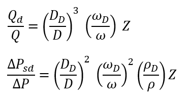
Performance changes due to these differences are scaled according to the Affinity Laws, which is a close approximation though not precise for compressible gases.
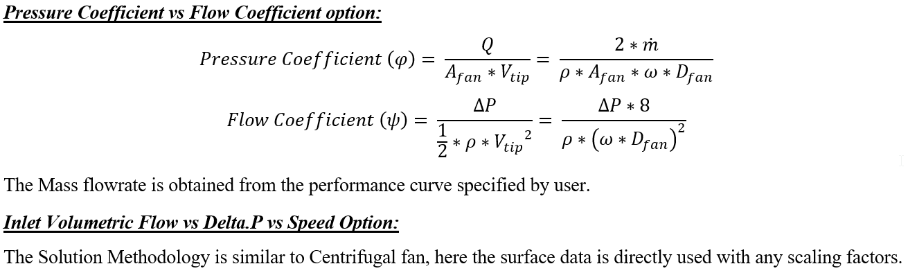
For Axial Fan, users provided Surface data “Volumetric Flow rate vs. Delta.P vs Speed” obtained from manufacturer. Since this Surface data consist of Fan Performance curves for various speeds, no scaling is used.
Axial Compressors models a simple compressor. The performance of the compressor is determined by its performance map. The map shows the relationship between the pressure ratio and volumetric or mass flow rate. The usable section of the map is defined by the Surge and Choke lines and the maximum compressor speed. The red lines show increasing compressor speeds.
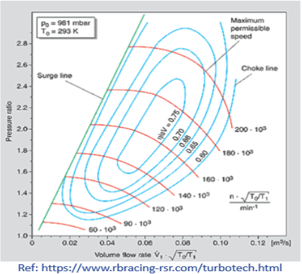
Surge Line
This is the point at which the air flow stalls at the compressor inlet. If the volume flow is too small or the pressure ratio is too high, then the air flow can longer adhere to the suction side of the compressor blades, which interrupts the discharge process. The air flow through the compressor is reversed until a stable pressure ratio with positive flow rate is reached. The pressure then builds up again and the cycle repeats itself. This flow instability continues at a fixed frequency and the resultant noise is referred to as 'surging'.
Choking Line
The maximum centrifugal compressor rate is normally limited by the cross-section at the compressor inlet. When the flow at the compressor wheel reaches sonic velocity, no further flow rate increase is possible. The choke line is shown in Figure 2 bisecting the descending compressor speed lines.
Axial Turbines models a simple Turbine. The performance of the turbine is determined by its performance map. The Typical turbine map below shows the relationship between the pressure ratio and volumetric or mass flow rate & Efficiency.
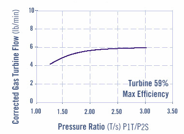
Fig: Turbine Performance Map
Fans, Compressors, and Turbine Element Inputs
Table of the inputs for the Fan and Compressor Element.
| Element Specific Fans and Compressors Element Input Variables | ||
| Index | Field | Description |
| 1 | Subtype (SUBTYPE) |
Fans & Compressors Subtype 1: Centrifugal Fan 2: Centrifugal Compressor 3: Axial Fan 4: Axial Compressors 5: Axial Turbine |
| 2 | Inlet Static Temperature (INLET_TS) | Temperature at the inlet to the fan/compressor |
| 3 | Inlet Static Pressure (INLET_PS) | Static pressure at the inlet to the compressor |
| 4 | Inlet Density (INLET_RHO) | Density of the gas at the inlet to the fan or compressor |
| 5 | Rotational Speed (DESIGN_SPEED) | Speed of the machine at the design conditions |
| 6 | Compresser/Fan Diameter (DESIGN_DIA) | Diameter of the Fan/compressor which will be used as a characteristic dimension for fan affinity calculations |
| 7 | Fixed Choking Flow rate (CHOKE_GPM) | Flow rate above which choking expected to occur |
| 8 | Fixed Surge Flow rate (SURGE_GPM) | Flow rate below which the machine is expected to become dynamically unstable |
| 9 | Inlet Pipe Diameter (IN_PIPE_DIA) | Inlet pipe diameter of the fan or compressor |
| 10 | Outlet Pipe Diameter (OUT_PIPE_DIA) | Outlet pipe diameter of the fan or compressor |
| 11 | Compresser/Fan Diameter (DIAMETER) | Diameter of the Fan/Compressor being used in the network |
| 12 | Speed (SPEED) | Rotational speed of the fan or compressor as used in the network |
| 13 | Efficiency (%) (FLAG) |
Efficiency Input Option 1: Fixed Efficiency For axial fan, centrifugal fan, and centrifugal compressor: 2: Polytropic Efficiency vs Inlet Volumetric Flow Rate For Axial compressor and turbine: 2: Polytropic Efficiency vs Corrected Flow Rate vs Pressure Ratio 3: Polytropic Efficiency vs Corrected Flow Rate vs Corrected Speed 4: Polytropic Efficiency vs Pressure Ratio vs Corrected Speed |
| 14 | Efficiency Value (EFFICIENCY) | Fan/Compressor Efficiency value in % |
| 15 | Pressure Rise Method (PS_RISE_METHOD) |
Options to Specify Delta-P Terms
|
| 16 | Swept Area (SWEPT_AREA) |
Swept Area of Fan (Used for Subtype:3 Axial Fan & Performance Data:2) |
| 17 | Performance Curves (PERFORM_DATA) |
Used for Subtype:3 Axial Fan 1: Pressure Coefficient vs Flow Coefficient 2: Volumetric Flow Rate vs Delta.P vs Speed |
| 18 | Mass or Volume (MASS_OR_VOL) |
Option to specify Mass flow rate or Volumetric flow rate (Used for Subtype: 4 Axial Compressor) |
| 19 | Choking Flow rate (CHK_OPT) |
Choking Flow rate Input Option 0: Fixed Choking Volumetric Flow rate 1: Choking Volumetric Flow rate vs Speed 2: Fixed Choking Corrected Mass Flow rate 3: Choking Corrected Mass Flow rate vs Corrected Speed |
| 20 | Surge Flow rate (SUR_OPT) |
Surge Flow rate Input Option 0: Fixed Surge Volumetric Flow rate 1: Surge Volumetric Flow rate vs Speed 2: Fixed Surge Corrected Mass Flow rate 3: Surge Corrected Mass Flow rate vs Corrected Speed |
| 21 | Efficiency Calculation (EFF_METHOD) | The method used to calculate the exit temperature of the element.
0: Auto (default). Option 2 is used if real gas or the energy
equations use enthalpy. Otherwise, option 1 is used.
|
Fans, Compressors, and Turbine Theory Manual
| Nomenclature: | |
| A: Orifice mechanical area | R: Gas Constant |
| Q: Volumetric Flow Rate | Ts: Static Temperature |
| Density | |
| Tt: Total Temperature | M: Mach Number |
| Pt: Total pressure | Cp: Specific Heat |
| Ps: Static pressure | gc: gravitational constant |
| Z: Temperature Correction Factor | |
| Subscripts: | |
| in, up, 1: Upstream station | d: Design Point |
| ex, dn, 2: Downstream station | Ref: Reference Conditions |
Centrifugal Fan and Centrifugal Compressor:
Performance changes due to these differences are scaled according to the Affinity Laws, which is a close approximation though not precise for compressible gases.
Solution Methodology:
- Actual Inlet Flow Rate at current operating conditions is converted to equivalent flow at the Design Point, using the Affinity Laws, the flow is limited to lie between Surge Flow Rate and Choking Flow Rate and performance characteristics are read at that Flow Rate.
- The Pressure (Difference) and Power read from the curves are then converted back to actual values at current operating conditions for use in the simulation or results.
- In a Fan or Compressor, mechanical losses are assumed to be small relative to the conversion loss in the impeller at Design Speed, so Polytropic Efficiency is treated as Overall Efficiency in these models.
- At the Choking limit & Surge Limit, system flow rate is limited to Choking Flow Rate & Surge Flow Rate respectively, scaled according to the affinity laws.
The Actual inlet Mass flow rate is determined by following procedure.,
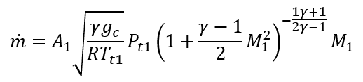
For Centrifugal Compressor,
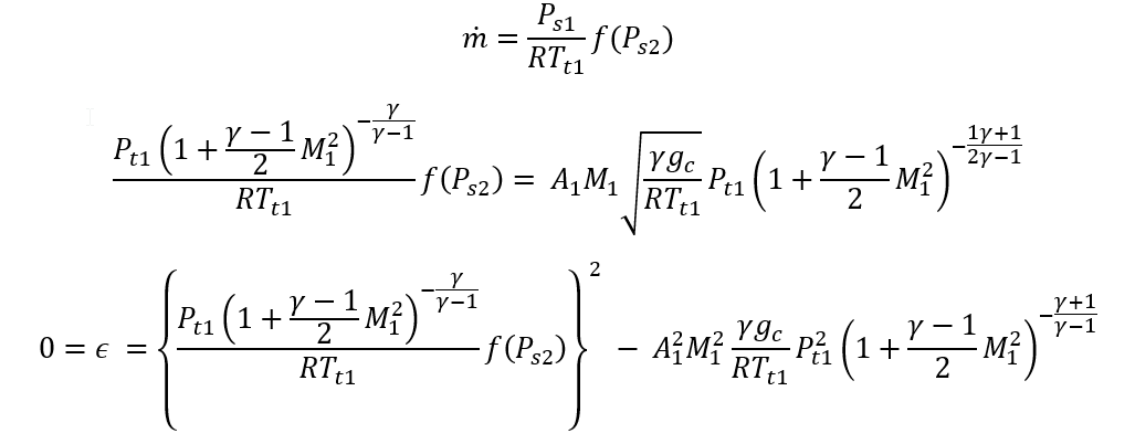
Newton-Raphson method is used to solve above mentioned coupled continuity and momentum equations to Mass Flow rate.
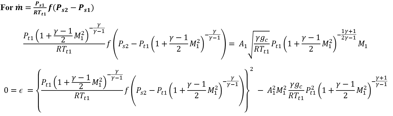
For Fan Centrifugal,
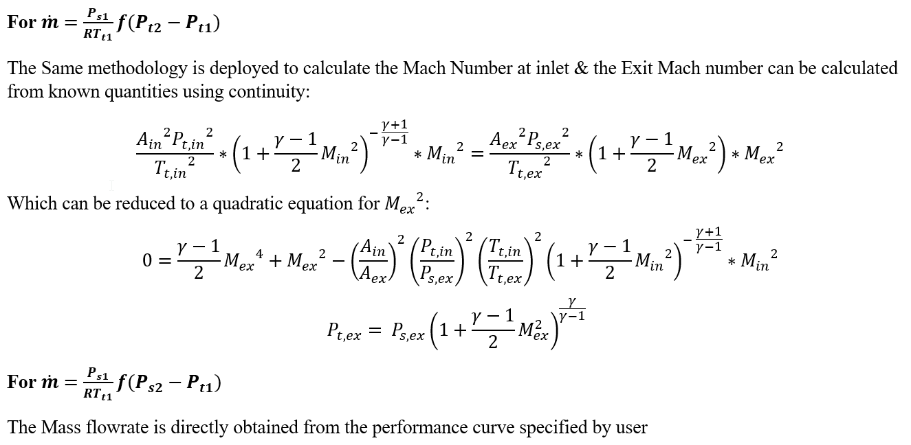
Axial Fan
Axial Compressors
The Mass flow rate is obtained from the user-supplied performance curve specified.
The Outlet Total Temperature, Tt2, is estimated using the polytropic efficiency and pressure rise. The equations are based on the efficiency calculation method. All methods, other than the ideal gas method, require fluid properties from Coolprop. The Schultz and Small Step methods are described in references 1 and 2.
Efficiency method = ideal gas
Efficiency method = Schultz
m is an exponent derived from the fluid properties and polytopic efficiency.
Efficiency method = Small Stage Step (and Fine)
The small step methods are the same except for the number of steps. The Small Step method uses the number of steps for a pressure ratio of 1.055, and the Small Step Fine method uses 100 steps.
- Use upstream Pt and Ht (actual enthalpy) to get the entropy.
- Use the Pt at the end of the step and entropy from 1 to get the enthalpy for the isentropic process.
- Use the definition of the polytropic efficiency to get the actual enthalpy at the end of the step. Polytropic efficiency=isentropic enthalpy change/actual enthalpy change.
- Repeat steps 1-3 for each step.
Axial Turbines
The Mass flow rate is obtained from the user-defined performance curve.
The Outlet Total Temperature, Tt2, is estimated using the polytropic efficiency and pressure rise. The equations are based on the efficiency calculation method. All methods, other than the ideal gas method, require fluid properties from Coolprop. The Schultz and Small Step methods are described in references 1 and 2.
Efficiency method = ideal gas
The Schultz and Small Step methods are similar to the compressor with modifications for pressure decrease in the turbine.
Fans, Compressors, and Turbine Element Outputs
The following listing provides details about Fans & Compressor element output variables.
| Name | Description | Units |
|---|---|---|
| SUBTYPE | Fans and Compressors Subtype 1: Centrifugal Fan 2: Centrifugal Compressor 3: Axial Fan 4: Axial Compressors 5: Axial Turbine (An echo of the user input) |
(None) |
| INLET_AREA | Inlet pipe area of the fan or compressor (An echo of the user input) | In2, m2 |
| OUTLET_AREA | Exit pipe area of the fan or compressor (An echo of the user input) | In2, m2 |
| FAN/COMPRESSOR_DIA |
Diameter of Fan/Compressor (Usually an echo of the user input unless modified inside Flow Simulator.) |
in, m |
| DESIGN_DIA |
Design Diameter (An echo of the user input) |
in, m |
| RPM |
Operating Speed (Usually an echo of the user input unless modified inside Flow Simulator.) |
RPM |
| DESIGN_SPEED | Design Speed | RPM |
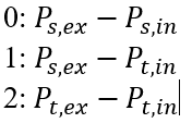
| LOSS_COEFFICIENT | (PTIN-PTEX)/(PTIN-PSIN) | (None) |
| EFFICIENCY | Fan/Compressor Efficiency | (None) |
| POWER | 231.0D0 / 60.0D0 / 12.0D0 / 550.0D0 * INLET_GPM * (PTEX - PTIN) | HP, W |
| HEAT_DUTY | POWER * (745.69987/0.293071) * (1-POLY_EFF)/1000 | HP, W |
| PTS | Driving pressure relative | psia, MPa |
| PSIN | Inlet Static pressure | psia, MPa |
| PTEX | Exit Total pressure relative | psia, MPa |
| PSEX | Exit Static pressure | psia, MPa |
| PSEB | Effective sink (static) pressure | psia, MPa |
| TTS | Inlet Total temperature of fluid | deg F, deg K |
| TSIN | Inlet Static temperature | deg F, deg K |
| TTEX | Exit Total temperature | deg F, deg K |
| TSEX | Exit Static temperature | deg F, deg K |
| INVEL | Inlet Velocity | ft/s, m/s |
| INMN | Inlet Mach number | (unitless) |
| INREYN | Inlet Reynolds number | (unitless) |
| EXVEL | Exit Velocity | ft/s, m/s |
| EXMN | Exit Mach number | (unitless) |
| EXREYN | Exit Reynolds number | (unitless) |
References
- Evans B.F., Huble, S., "Centrifugal Compressor Performance, Making Enlightened Analysis Decisions", Turbomchinery and Pump Symposia, 2017.
- Schultz, J. M. (1962). The polytropic analysis of centrifugal compressors. Journal of Engineering for Power, 84(1), 69–82.