SS-T: 4035 Thermal Transient Analysis
Tutorial Level: Intermediate Perform a thermal transient analysis.
- Prerequisites
- Some features used in this tutorial are only available in the SimSolid Advanced version. Switch to Advanced to complete this tutorial.
- Purpose
- SimSolid performs meshless
structural analysis that works on full featured parts and assemblies, is
tolerant of geometric imperfections, and runs in seconds to minutes. In this
tutorial, you will do the following:
- Learn how to perform thermal transient analysis in SimSolid.
- Model Description
- The following file is needed for this tutorial:
- fin2.x_b
-
Figure 1. 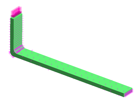
Import Geometry
- Open a new SimSolid session.
-
Click Import from file
 .
.
- In the Open geometry files dialog, choose fin2.x_b.
-
Click Open.
The assembly will load in the modeling window.
Apply Material
Thermal transient analysis requires a specific heat capacity. Add a new material or edit an existing material to add the required values.
- In the main menu, click .
- In the Define material database dialog, click Edit current.
- In the Material database dialog, under the Generic Materials group, right-click Steel and select Copy from the context menu.
-
Edit the Steel - Copy thermal properties.
- Click Edit material.
- For thermal conductivity, enter 73 W/m k.
- For Specific heat transfer to 508 J/Kg k.
- Click Apply.
- Click Save.
- Close the Material database dialog.
- In the Project Tree, click on the Assembly branch.
-
On the Assembly workbench, click Apply
material
 .
.
- In the dialog, select the newly created material and click Apply to all parts.
- Click Close.
Create Thermal Transient Analysis
-
On the main window toolbar, select Thermal
 > Thermal Transient
  .
The new analysis appears in the Project Tree.
.
The new analysis appears in the Project Tree. - For Time span, enter 500 sec.
- Set the number of output timesteps to 50.
- For Initial temperature, enter 0 C.
- Click OK.
Create Time Functions
- In the Project Tree, select Transient thermal 1 to open the Analysis Workbench toolbar.
-
Create the uniform time function.
-
On the workbench toolbar, click Time function
 .
.
- In the Time function dialog, click Standard.
- In the Standard time functions dialog, for Function type, select Uniform from the drop-down menu.
- Click OK.
- Review the plot in the Time function dialog and click OK.
- In the Project Tree, right-click on the time function and select Rename.
- For name, enter uniform.
-
On the workbench toolbar, click Time function
-
Create the Linear time function.
-
On the workbench toolbar, click Time function
.
-
On the workbench toolbar, click Time function
Apply Heat Flux
-
On the Analysis Workbench toolbar, click
Flux
 .
.
-
Select the faces highlighted in Figure 2.
Figure 2. 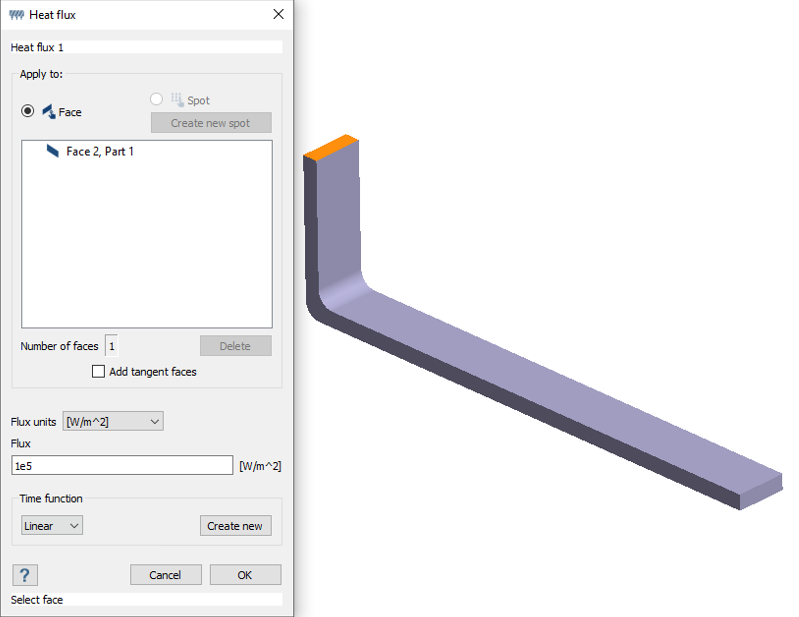
- For Flux, enter 1e5.
- For Time function, select Linear from the drop-down menu.
- Click OK.
Apply Thermal Convection
-
On the Analysis Workbench toolbar, click
Convection
 .
.
-
Select the faces highlighted in Figure 3 (all faces except the one with heat flux applied).
Figure 3. 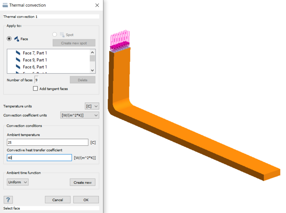
- For Ambient temperature, enter 25 C.
- For Convective heat transfer coefficient, enter 40 W/m^2*K.
- For Ambient time function, select Uniform from the drop-down menu.
- Click OK.
Edit Solution Settings
- In the Analysis branch of the Project Tree, double-click on Solution settings.
- In the Solution settings dialog, for Adaptation select Global+Local in the drop-down menu.
- Click OK.
Run Analysis
- On the Project Tree, open the Analysis Workbench.
-
Click
 Solve.
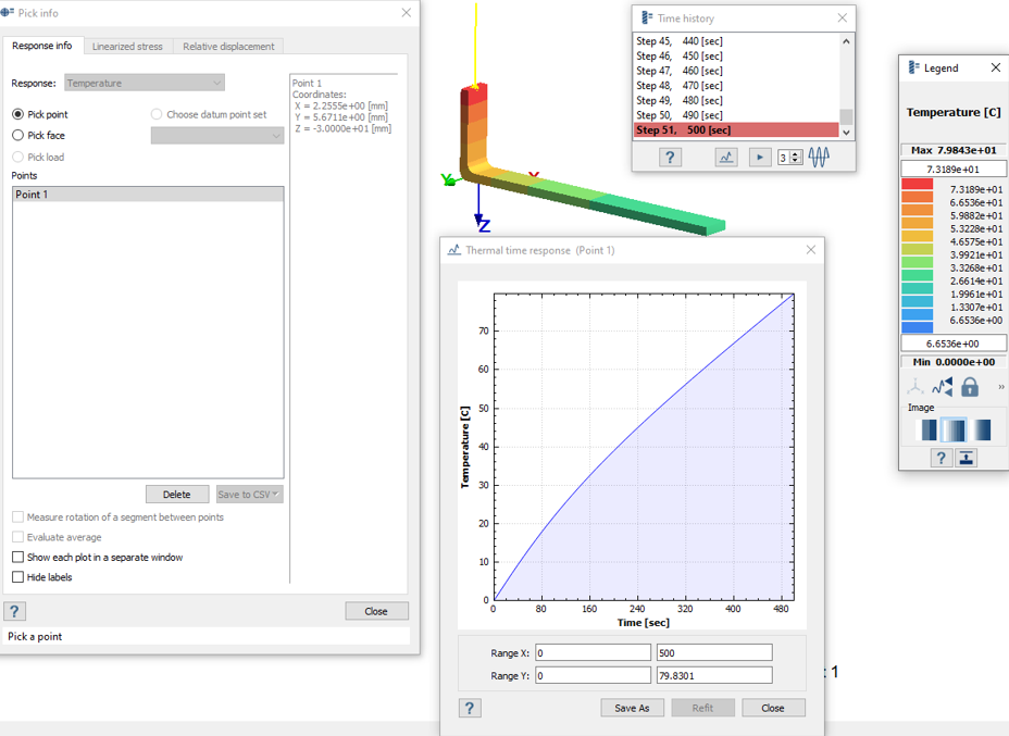
Review Results
- In the Project Tree, select the Thermal transient 1 subcase.
-
On the Analysis Workbench, select Results plot
 > Temperature.
-
The Legend and Time History windows
appear and the modeling window displays the contour plot.
Figure 4. 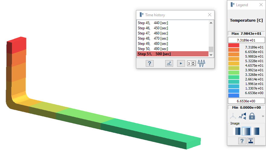
- In the Time history window, select the step to view the corresponding temperature plot.
-
Click
 (Show history
graph) to view a plot of thermal time response.
(Show history
graph) to view a plot of thermal time response.
-
Click
 (Animate
history) to animate the time history step by step.
Steps highlighted in blue and red in the Time history window indicate the steps with max and min temperatures.
(Animate
history) to animate the time history step by step.
Steps highlighted in blue and red in the Time history window indicate the steps with max and min temperatures.
Plot Response
Plot the response at regions of interest.
-
On the Analysis Workbench, select Pick
info
 .
.
-
Select any point on the model.
A thermal time response plot is shown at the selected point.
Figure 5.