SS-T: 4070 Random Response Analysis
Create random response analysis in SimSolid.
- Purpose
- SimSolid performs meshless structural
analysis that works on full featured parts and assemblies, is tolerant of
geometric imperfections, and runs in seconds to minutes. In this tutorial,
you will do the following:
- Create dynamic random analysis for a walkway assembly with base excitation load.
- Model Description
- The following files are needed for this tutorial:
- Random.ssp
- PSD_Function.csv
-
Figure 1. 
Open Project
- Start a new SimSolid session.
-
On the main window toolbar, click Open Project
 .
.
- In the Open project file dialog, choose Random.ssp
- Click OK.
Create Modal Analysis
-
On the main window toolbar, click the
 (Modal analysis) icon.
- In the popup Number of modes window, specify the number of modes as 9.
-
Click OK.
The new modal analysis appears in the Project Tree.
Create Immovable Support
-
In the Analysis Workbench, click Immovable
Support
 .
.
- In the dialog, verify the Faces radio button is selected.
-
In the modeling window, select the two faces shown in
Figure 2.
Figure 2. 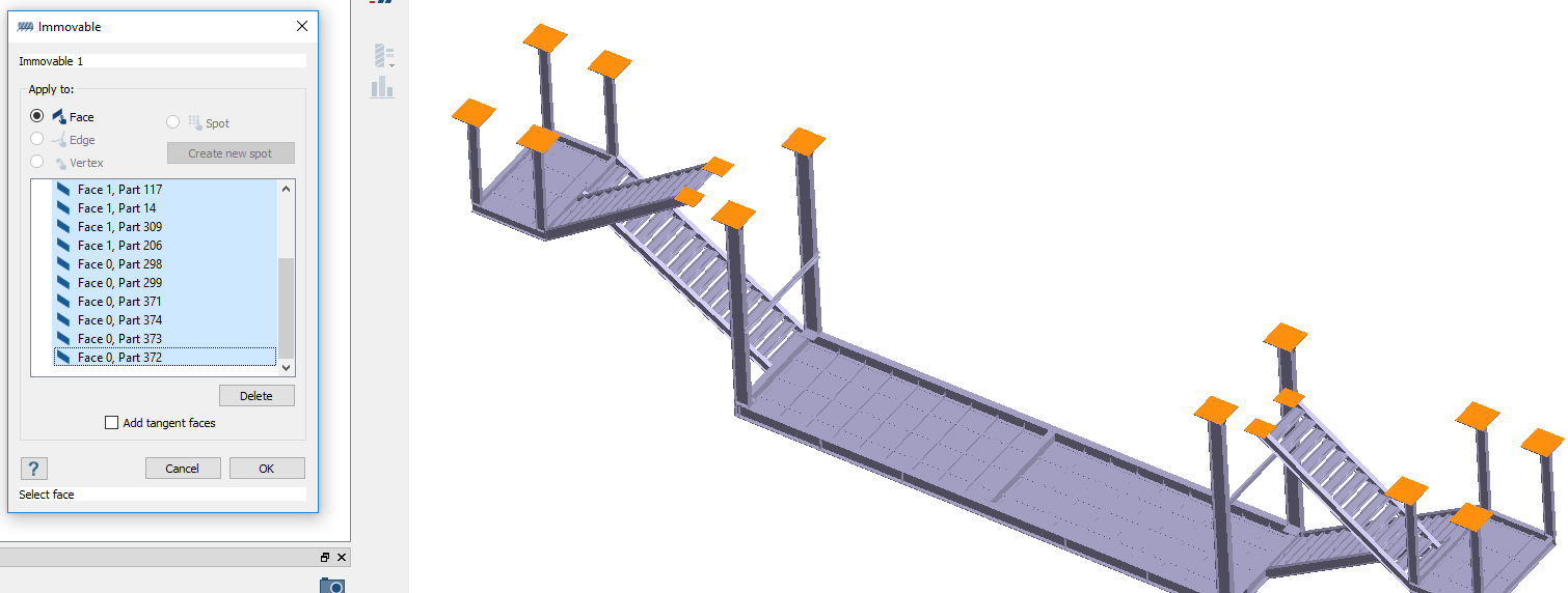
-
Click OK.
The new constraint, Immovable 1, appears in the Project Tree. A visual representation of the constraint is shown on the model.
Edit Solution Settings
- In the Analysis branch of the Project Tree, double-click on Solution settings.
- In the Solution settings dialog, for Adaptation select Global+Local in the drop-down menu.
- Click OK.
Run Analysis
- On the Project Tree, open the Analysis Workbench.
-
Click
 (Solve).
Review Results
- In the Project Tree, Select the Modal 1 subcase.
-
On the Analysis Workbench, select
 > Displacement Magnitude.
The Legend window opens and displays the contour plot. The Frequency (Hz) window opens and lists the modes.
> Displacement Magnitude.
The Legend window opens and displays the contour plot. The Frequency (Hz) window opens and lists the modes.Figure 3. 
Create Random Response Analysis
-
On the main window toolbar, select
 > Random response.
The Dynamic random response setup dialog opens. Link to the available Modal analysis result.
> Random response.
The Dynamic random response setup dialog opens. Link to the available Modal analysis result. - For Frequency span, accept the default values for the Lower limit, 2.35517, and the Upper limit, 11.5542.
- Select the Modal damping tab.
- Set the Default damping ratio to 0.03.
- Click OK.
Create PSD Functions
- In the Project Tree, click on the Assembly branch to open the Assembly workbench.
-
On the workbench toolbar, click the
 (Power Spectral Density function) icon.
-
In the dialog, click the Import CSV button.
Figure 4. 
-
In the File explorer, browse to the PSD_Function.csv file
and click Open.
The function is plotted in the XY graph in the dialog.
Figure 5. 
Define Loads
-
On the Assembly workbench toolbar, click the
 (Base excitation) icon.
- In the dialog, ensure Excitation type is set to Acceleration.
- Ensure Units are set to [m/sec^2].
- For Amplitude, enter 10.
- For direction, enter 1 for X, Y, and Z.
- Click OK.
Run Analysis
- On the Project Tree, open the Analysis Workbench.
-
Click (Solve).
Review Results
- In the Project Tree, Select the Dynamic random 1 subcase.
-
On the Analysis Workbench, select > Displacement Magnitude.
The Legend window opens and displays the contour plot. The Dynamics random response window opens. Use the slider to animate frequencies.
Figure 6. 
Plot Response Curve
-
On the workbench toolbar, click the
 (Pick info) icon.
- Verify the Pick point radio button is selected.
-
In the modeling window, select a point on the model as
shown in below.
Figure 7. 
-
Click Evaluate.
The response for the point is plotted in the XY graph in the dialog. Use the scroll wheel to zoom in, the left mouse button to pan, or the Refit button to reset the graph.
Figure 8. 
-
Obtain partial response.
-
In the dialog, pick a point on the curve to show the Modes
contributions into response table.
Figure 9. 
The plot in the dialog updates to show the partial response. -
In the dialog, pick a point on the curve to show the Modes
contributions into response table.