SS-T: 4100 SN Time - Import Loadcase - Channel Mapping
Import channels and create events automatically using a .csv file.
Prerequisites
Some features used in this tutorial are only
available in SimSolid Advanced version. Please
switch to Advanced to complete this tutorial.
Purpose
SimSolid performs meshless structural
analysis that works on full featured parts and assemblies, is tolerant of
geometric imperfections, and runs in seconds to minutes. In this tutorial,
you will do the following:
Create SN Time Fatigue loadcase.
Import channels and create events automatically with a .csv
file.
Define channel mapping for events.
Review results.
Model Description
The following model files are needed for this tutorial:
SNTime-ChannelMapping.ssp
ChannelMapping.csv
Figure 1.
The project (.ssp) file has the following
specifications:
Material is set to Steel for all parts.
Multi-loadcase workbench is included. Learn more about creating
multi-loadcases here.
Load cases with remote loads are included.
Open Project
Start a new SimSolid session.
On the main window toolbar, click Open Project.
In the Open project file dialog, choose
SNTime-ChannelMapping.ssp
Click OK.
Review Model
In the Project Tree, expand the
Multi-loadcases 1Analysis Workbench.
Review the loads.
Figure 2.
Click (Results plot) and choose the desired plot to
review the stresses for each loadcase.
Add Fatigue Material Properties
If an SN curve has already been assigned, skip this step. Check the assigned material
properties by right-clicking Assembly in the Project Tree and selecting Show > Materials.
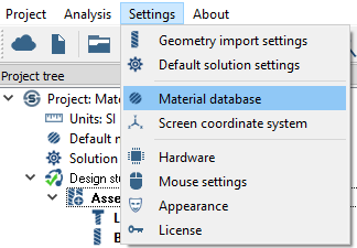
In the main menu, click Settings > Material database.
Figure 3.
In the Generic Materials group, right-click Steel and select
Copy from the context menu.
Edit the copied material.
Select Steel1 - Copy_0.
Click Edit material.
Add fatigue curves.
In the editing field of the dialog, expand the Fatigue
properties branch and click Add stress-life
(SN) curve....
Verify the Curve definition method is set to Estimate from
UTS.
Click Apply.
Click Save.
Create SN Time Analysis
On the main window toolbar, click
(Fatigue analysis).
In the drop-down menu, select SN Time.
The new analysis appears in the Project Tree.
The SN Time Workbench items are listed.Figure 4.
Import Loadcase and Channel Map
In the Project Tree, open the
Fatigue SN/EN Time Workbench.
On the workbench toolbar, click (Import loadcase-channel map).
In the dialog, for Map to, verify Multi-loadcases 1 is
selected.
Click Set Path and pick the path for the load history
files.
Figure 5. These can be rsp or rpc files.
Click Import from CSV and select
ChannelMapping.csv.
Figure 6.
Note: You cannot edit the events from the dialog. Make necessary changes to the
.csv file before import.
Click OK.
Imported Loadcase-channel Map File Format
CSV file format for importing loadcase-channel map files.
CSV file format fields
Figure 7. The fields in the .csv file are the same as those in the dialog.
Event name – Alpha-numeric values. Name of the event.
Repeats – Numeric values. Event repeats.
Gate range (optional) – Numeric values. Relative fraction of maximum
gate range. The reference value is the maximum range multiplied by gate
range and used for gating out small disturbances or "noise" in the time
series.
Filename – The RSP/RPC filename. Other file formats are not
supported.
Channel sets - The loadcase-channel map sets.
If empty, maps based on the order of channels and load cases.
1st loadcase is mapped to 1st channel, 2nd loadcase to 2nd
channel and so on until the last loadcase/channel.
If there is an input in channel sets, mapping is based on the
user input. For example, if the input is 2-4;6. It translates to
the 1st three loadcases being mapped to channels 2 to 4, and the
4th loadcase being mapped to the 6th channel.
In this case, the input is 2:1. The 1st loadcase is mapped to the 2nd channel
and the 2nd loadcase is mapped to the 1st channel. The 3rd loadcase has no
mapping.
Review Channels
In the Project Tree, double-click on a channel.
The Channel group dialog opens and lists the
channels available in the load history file, along with their plots and
coordinates. You can cycle between them to view the plots.
Note: You cannot edit
channels from this dialog.
Figure 8.
Optional: Click on the column headers to sort the plot table by Time or Amplification
Factor.
Click Cancel to close the window.
Review Events
In the Project Tree, double-click on an event.
The Event setup dialog opens. You can edit channel
mappings, scale, offset, gate range, and event repeats from this dialog. You can
also add new Channel-loadcase mapping by clicking Add
row.
Keep the Channel scale as 1 for Event 1 and Event 2, as
shown in the figures below.
Note: Event 1 has default mappings as defined. Event 2 has manually defined
mappings. The second channel is mapped to Loadase 1 and the first channel is
mapped to Loadcase 2.
Figure 9. Event 1 Figure 10. Event 2
Event 1 has default mappings as defined. Event 2 has user defined
mappings; the 2nd channel is mapped to Loadcase 1 and the 1st channel is mapped
to Loadcase 2.
Run Analysis
On the Project Tree, open
the Analysis Workbench.
Click (Solve).
Review Results
In the Project Tree, Select the Fatigue SN
Time 1 subcase.
On the Analysis Workbench, select > Fatigue damage.
The Legend window opens and displays the contour
plot. The Events window opens and lists all events. You
can plot damage for each event or plot cumulative damage.Figure 11.
Pick info.
On the Results Workbench toolbar, click (Pick info).
In the modeling window, select points of
interest.
In the Pick info dialog, for Event, select Total
from the drop-down menu to view cumulative damage, or select the
individual Event of interest.

 .
.

 (Results plot) and choose the desired plot to
review the stresses for each loadcase.
(Results plot) and choose the desired plot to
review the stresses for each loadcase.
 (Fatigue analysis).

 (Import loadcase-channel map).


 (Solve).

 (Pick info).
