Motion: Joint Based

Model ElementMotion_Joint defines a motion input at a degree-of-freedom in a joint.

Description

This input is allowed only on three types of joints:

Translational joints (translational motion).
Revolute joints (rotational motion only).
Cylindrical joints (either rotational or translational).
Point-To-Curve (parametric-curve motion).

Define an expression for the motion characteristics. The expression may be used to define displacement, velocity, or acceleration. The expression is usually a function of time. See Comment 8 if you want to make the motion expression dependent on system states.

A translational motion is defined in one of the following ways:

DZ(I,J,J) - expression = 0 to Translational Displacement Motion
VZ(I,J,J,J) - expression = 0 to Translational Velocity Motion
ACCZ(I,J,J,J) - expression = 0 to Translational Acceleration Motion

A rotational motion may be defined in one of the ways listed below:

AZ(I,J) - expression = 0 to Rotational Displacement Motion
WZ(I,J,J) - expression = 0 to Rotational Velocity Motion
WDTZ(I,J,J,J) - expression = 0 to Rotational Acceleration Motion

A parametric-curve motion may be defined in one of the following ways:

Distance traveled along the curve = expression to Displacement Motion
Velocity traveled along the curve = expression to Velocity Motion
Acceleration traveled along the curve = expression to Acceleration Motion

In the above, I is the i_marker_id of the joint and J to the j_marker_id. The software defines the state dependent term in the equations and you define the expression, the type of motion, and the joint on which the input is to be provided.

For a translational motion, the z-axis of j_marker_id defines the direction of positive motion. The origin of i_marker_id moves along this line. At zero displacement, the origins of the two markers are coincident.

For a rotational motion, i_marker_id rotates about the common z-axis. A positive motion results in counter clockwise rotation.

For a parametric-curve motion, the distance is measured from the initial point position on the parametric curve. The distance is positive along the direction of the curve when the parameter U increases, and negative along the opposite direction.

A reaction force is associated with each Motion_Joint. This reaction force tells the system the force or torque that is needed to apply the requested motion.

When the expression is a function of time, energy is either added to or removed from the system. Motion inputs may be considered as actuators or motors with infinite force or torque capacity.

The expression that you supply may be specified using either a MotionSolve expression, a user-defined subroutine, or a plant input.

If the motion input is constant over time, it can be simplified using the type = “CONSTANT”.

Format: Expression-based Motion

<Motion_Joint
       id            = "integer"
     [ label         = "string" ]       
       joint_id      = "integer"
       motion_type   = { "T" | "R" | "P" }
     [ is_virtual    = { "FALSE" | "TRUE" } ]
   {   
       val_type      = "D"
      |  
       val_type      = "V"
       ic_disp       = "real"
      |  
       val_type      = "A"
       ic_disp       = "real"
       ic_vel        = "real"
   }
   {   
       type          = "EXPRESSION"
       expr          = "motionsolve_expression"
      |
       type                    = "USERSUB"
       usrsub_dll_name         = "valid_path_name"
       usrsub_param_string     = "USER( [[par_1 [, ...][,par_n]] )"
       usrsub_fnc_name         = "custom_fnc_name"
      |
       type                    = "USERSUB"
       script_name             = "valid_path_name"   
       interpreter             = "string"
       usrsub_param_string     = "USER( [[par_1 [, ...][,par_n]] )"
       usrsub_fnc_name         = "custom_fnc_name"   
   } 
/>

Format: Plant Input-based Motion

<Motion_Joint
       id            = "integer"
     [ label         = "string" ]       
       joint_id      = "integer"
       motion_type   = { "T" | "R" | "P" }
       type          = "PLANT_INPUT"
       pinput_id     = "integer"
       val_index     = "integer"
/>

Format: Constant Motion

<Motion_Joint
       id            = "integer"
     [ label         = "string" ]       
       joint_id      = "integer"
       motion_type   = { "T" | "R" | "P" }
     [ is_virtual    = { "FALSE" | "TRUE"} ]
       type          = "CONSTANT"
   {   
       val_type      = "D"
       q             = "real"
      |  
       val_type      = "V"
       ic_disp       = "real"
       qd            = "real"
      |  
       val_type      = "A"
       ic_disp       = "real"
       ic_vel        = "real"
       qdd           = "real"
   }
/>

Attributes

id

Element identification number (integer>0). This number is unique among all Motion_Joint elements.

label

The name of the Motion_Joint element.

joint_id

Specifies the ID of the joint at which the motion input is applied.

motion_type

Specifies the type of motion that is to be applied. Motion types may be translational ("T"), rotational ("R"), or parametric-curve (“P”). Specify either "T", “R” or "P". Note that motions on translation joints are always of type "T". Motions on revolute joints are always of type "R". Motions on cylindrical joints may be of either type, but not both. Motions on Point-To-Curve are always tangential to the curve.

is_virtual(optional)

Defines whether the motion constraint is virtual or regular. If is_virtual is set to TRUE, the constraint is implemented as a virtual constraint. If is_virtual is set to FALSE, the constraint is implemented as a regular algebraic constraint.

The default is FALSE.

See Comments in Constraint_Joint for more information about virtual joints.

val_type

Specifies whether the motion applies a displacement input (D), a velocity input (V), or an acceleration input (A). You must select one value from "D", "V", or "A".

ic_disp

Specifies the displacement initial condition that is required when val_type = "V" or val_type = "A".

ic_vel

Specifies the velocity initial condition that is required when val_type = "A".

type

Select either "EXPRESSION", "USERSUB", "PLANT_INPUT", or “CONSTANT”. Specifies how the motion is defined. The EXPRESSION option specifies that the motion value is a MotionSolve expression that can be evaluated at run-time. The USERSUB option indicates that the value of the motion value is specified in a user defined subroutine. The parameters "usrsub_param_string" and "usrsub_dll_name" are used to provide more information about the user defined subroutine. The PLANT_INPUT option indicates that the Motion is used as a plant input. The “val_index” defines the enforcement level and “pinput_id” references the Control_PlantInput. The CONSTANT option is an alternative to EXPRESSION to define a motion with a constant value.

expr

Defines an expression that defines the motion value. Use this parameter only when type = EXPRESSION. Any valid run-time MotionSolve expression can be provided as input.

usrsub_dll_name

Specifies the path and name of the DLL or shared library containing the user subroutine. MotionSolve uses this information to load the user subroutine MOTSUB in the DLL at run time.

usrsub_param_string

The list of parameters that are passed from the data file to the user defined MOTSUB. Use this keyword only when type = USERSUB is selected.

usrsub_fnc_name

Specifies an alternative name for the user subroutine MOTSUB.

script_name

Specifies the path and name of the user written script that contains the routine specified by usrsub_fnc_name.

interpreter

Specifies the interpreted language that the user script is written in (example: "PYTHON"). See User-Written Subroutines for a choice of valid interpreted languages.

val_index

Defines the simultaneous enforcement of constraints at the position, velocity, and acceleration levels.

“3”: The motion is enforced only at the position level.
"2": The motion is enforced at the position and velocity level simultaneously.
"1": The motion is enforced at the position, velocity, and acceleration level simultaneously. See Motion: Marker Based.

pinput_id

Specifies the Control_PlantInput ID at which the motion input is applied.

q, qd, qdd

Specifies the constant position (q), velocity (qd), or acceleration (qdd). Only valid if type = “CONSTANT”.

Example

The first example shows how experimental data may be fed into the system as motion input.

Automotive vehicle handling simulations are often performed using semi-analytical simulation techniques. A vehicle to be tested is instrumented with sensors to measure the steering wheel angle while it is being driven. The vehicle is driven on the proving grounds. The driver may perform a variety of maneuvers simulating real-life steering situations. This data is collected as a function of time.

The experimental data is "cleaned" to remove noise and high frequency content. Next, a vehicle model suitable for vehicle handling studies is created in MotionSolve. The experimental data is modeled as a SPLINE in MotionSolve and it is provided as steering input to the analytical model of the vehicle. During the simulation vehicle behavior necessary for evaluating handling are collected.

The steering input, after being "cleaned", might look as shown in Figure 1:

Figure 1. Experimentally measured steering input

The Motion_Joint for the steering input would like this:

<Motion_Joint
     id                  = "1"
     joint_id            = "301"
     motion_type         = "R"
     val_type            = "D"
     type                = "EXPRESSION"
     expr                = "CUBSPL(Time, 0, 301001)" >
</Motion_Marker>

The second example demonstrates how you may specify the motion of a worm and wheel mechanism using a Motion_Joint. The image below illustrates the mechanism.

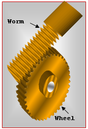
The worm gear is driven by a motor at a constant rate of 200 revolutions per second. Due to the gearing ratio, the wheel turns slowly relatively to the worm. This is a speed reduction system ideally forming part of a drive or lifting device. Constraint_Joint 101 defines a revolute joint between the worm gear shaft and the housing. A Motion_Joint on this revolute joint simulates the motor. The motion definition would look as follows:

<Motion_Joint
     id                  = "2"
     joint_id            = "101"
     motion_type         = "R"
     val_type            = "D"
     type                = "EXPRESSION"
     expr                = "200*2*PI*Time" >
</Motion_Joint>

Comments

Three constraints are added for each Motion_Joint: one in the displacement domain, the second in the velocity domain and the third in the acceleration domain.
- When a displacement constraint is specified, the velocity and acceleration constraints are obtained by analytically differentiating the displacement constraints.
- When a velocity constraint is specified by the user, the displacement constraint is obtained by numerically integrating the velocity constraint and the acceleration constraint by analytically differentiating the velocity constraint.
- When an acceleration constraint is specified, the velocity constraint is obtained by numerically integrating the acceleration constraint, and the displacement constraint by numerically integrating the velocity constraint.
Differentiation tends to amplify any noise in the input signal. It is therefore important to ensure that all expressions and experimental data provided as input be smooth. More precisely, they must have continuous first and second time derivatives. Avoid the AKISPL() interpolation method when interpolating experimental data. AKISPL()does not calculate good first and second derivatives. Use CUBSPL() instead.
Integration tends to decrease the noise in an input signal. Therefore, it is a good idea to use velocity inputs when providing interpolated experimental or tabular data as motion input expressions.
Define your curve with as few points as possible. Excessively large number of interpolation points in a cubic curve makes its first derivative "jumpy", and its second derivative "extremely jumpy", even though the curve itself may look smooth.
Make sure that the initial velocity of the motion matches the initial velocities of the bodies that it affects. For example, if your mechanism simulation starts from an initial static state, then you should make sure that the input motion has zero initial velocity. The motion input overrides body and joint initial velocities if they are in conflict.
If you decide to use velocity inputs, be aware that the position is satisfied only to the integration error specified in the Param_Transient element. Likewise for acceleration inputs, the velocity and position are only satisfied to the integration error specified. Therefore, you may see some drift from the analytical solution. This is a limitation of any scheme based on numerical integration.
It is useful to take a look at the reaction force/torque time histories due to the motion constraint. It tells you how much force/torque is needed to achieve the given motion. You should ascertain whether or not this is realistic. Furthermore, it sometimes makes better physical sense to replace the motion with applied forces coupled with control laws. Remember that motion in a dynamic analysis is treated as a "hard" constraint with no room for compliance.
Motions can be defined as a function of either time or other states when using the DSTIFF integrator.
However, if VSTIFF, MSTIFF or ABAM are used, then the motions may only be functions of time. To define the motions as a function of state, you must apply a time lag to the system data you are requesting and then smooth it as discussed below.
- Assume that a Motion_Joint is used to apply a displacement that is based on the sensed radial velocity between two Reference_Markers 100 and 200. Then, you must code the user subroutine to implement the following:
  EXPR(T_k+1) = VR(100,200) evaluated at T_k,
  
  T_k+1- T_k is the sampling period for the system.
  Note that EXPR(T_k+1) is constant. However it changes whenever the velocity VR() is sampled. This implementation is not adequate because the sampled values are not continuous. You must fit a curve through the previously sampled values and extrapolate the curve to provide a smooth value. This is shown symbolically below:
```
EXPR(T_k+1) = CUBIC(VR(100,200)|_Tk, VR(100,200)|_Tk-1, VR(100,200)|_Tk-2)
```