
Control: FMU
Model ElementFMU (Functional Mock-up Unit) is an abstract modeling entity that defines a generic modeling element in MotionSolve.
Description
A standard, tool-independent interface, the Functional Mock-up Interface (FMI) defines the interface for accessing data from and depositing data into the FMU. MotionSolve uses the FMI to import one or more FMUs into a system model, connect these to other modeling components, and generate the combined model for solution.
Format
<FMU
     id                         = integer
     label                      = string
     full_label                 = string
     type                       = string
     path                       = string
     x_array_id                 = integer
     y_array_id                 = integer
     u_array_id                 = integer
     ic_array_id                = integer
     num_state                  = integer
     num_output                 = integer
     is_static_hold             = Boolean
     error_tol_factor           = real
     usrsub_dll_name            = string
     usrsub_fnc_name            = string
     var_name                   = string
     var_ic                     = string
     ip_address                 = string
     fmu_communication_interval = real
     start_time                 = real
/>
Attributes
- id
- Element identification number. This number is unique among all
FMUs.
- Integer > 0
- label
- The “short” name for the FMU element.
- String
- full_label
- The full name of the FMU element (usually the
MotionView system name).
- String
- type
- Type of FMU. Options include
“CoSimulation” or
“ModelExchange”.
- String
- Default: “ModelExchange”
- x_array_id
- Specifies the ID of the Reference_Array used to store
the continuous states, x, of this
FMU.
- Integer
- Default: None
- y_array_id
- Specifies the ID of the Reference_Array used to store
the output, y, of this FMU.
- Integer
- Default: None
- u_array_id
- Specifies the ID of the Reference_Array used to store
the input u of this FMU.
- Integer
- Default: None
- ic_array_id
- Specifies the ID of the Reference_Array used to store
the initial conditions for the continuous states,
x, of this FMU.
- Integer
- Default: None
- is_static_hold
- A flag for indicating whether the value of dynamic state is kept
constant during static or quasi-static simulations.
- Boolean
- Default: FALSE
- Applicable only to Model-Exchange FMUs
- error_tol_factor
- Integration error tolerance scale factor for the continuous states in an
FMU with type = ModelExchange.
- Real > 0
- Default: 1.0
- Applicable only to Model-Exchange FMUs
- num_state
- Number of continuous states in the FMU.
- Integer > 0
- Applicable only to model exchange FMUs.
- num_output
- Number of outputs from the FMU,
- Integer > 0
- usrsub_dll_name
- Specifies the path and name of the DLL or shared library that will be
used to load the FMU. MotionSolve uses this information
to load the user subroutine in the DLL at run time.
- String
- Default: “nugsefmu”
- usrsub_fnc_name
- Specifies the name for the user subroutine in the DLL for the FMU.
- String
- Default: “GSESUB”
- var_name
- String that lists the name of each variable inside FMU that can be
assigned a value.
- String
- Values delimited by “;” (semicolon)
- Default: None
- var_ic
- String that lists the value for each variable defined by
“var_name” that needs to be set by the user.
- String
- Values delimited by “;” (semicolon)
- Default: None
- ip_address
- IP address for the FMU connecting to MotionSolve.
- String
- Default: “PIPE”
- fmu_communication _interval
- The time interval between successive communications with the FMU of
type = CoSimulation. FMU outputs
are interpolated for all other calls.
- Real
- Default: HMAX, the maximum step size defined for the simulation by the simulation control parameters.
- start_time
- The start time for the coupled co-simulation, meaning MotionSolve simulates the system without the FMU of
type = CoSimulation from T0
(start time) to T (coupling time).
- Real
- Default: 0
- Applicable only to CoSimulation FMUs.
Example 1 - Model-Exchange type of FMU
In this example, an FMU of type “ModelExchange” is used in a MotionSolve analysis. The FMU has 12 inputs, 3 states and 6 outputs. Both MotionSolve and the FMU are operating on the same machine.
<!--Define the FMU below →
<FMU
     id                  = "1000"
     path                = "/staff/jwitt/work/Active_Damper_ME.fmu"
     type                = "ModelExchange"
     x_array_id          = "100"
     y_array_id          = "200"
     u_array_id          = "300"
     ic_array_id         = "400"
     error_tol_factor    = "0.8"
/>
<!--Define the FMU States as a solver Array of type X →
<Reference_Array
id = "100"
label = "FMU States"
type = "X"
num_element = "3"
/><!--Define the FMU Output as a solver Array of type Y →
<Reference_Array
id = "200"
label = "FMU Outputs"
type = "Y"
num_element = "6"
/><!--Define the FMU inputs as a solver Array of type U →
<Reference_Array
id = "300"
label = "FMU Inputs"
type = "U"
num_element = "12"
501 601 701 801 901 1001 1101 1201 1301 1401 1501 1601
/><!--Define the ICs for the FMU states in a solver Array →
<Reference_Array
id = "400"
label = "FMU Initial Conditions"
type = "IC"
num_element = "3"
1.456 0.8264 234.321
/>Example 2: Co-Simulation type of FMU
In this example, an FMU of type “CoSimulation” is shown. It takes 6 inputs and provides 18 outputs. These are defined in arrays of type U and Y, respectively. MotionSolve is running on a machine with the IP address 172.16.0.8.
<!-- Define the FMU below -->
<FMU
     id                  = "1000"
     path                = "/staff/jwitt/work/Active_Damper_CS.fmu"
     type                = " CoSimulation"
     y_array_id          = "200"
     u_array_id          = "300"
     ip_address          = "172.16.0.8"
/>
<!--Define the FMU Output as a solver Array of type Y-->
<Reference_Array
id = "200"
label = "FMU Outputs"
type = "Y"
num_element = "18"
/><!-- Define the FMU inputs as a solver Array of type U-->
<Reference_Array
id = "300"
label = "FMU Inputs"
type = "U"
num_element = "6"
501 601 701 801 901 1001
/>Comments
- The Functional Mock-Up Interface
Functional Mock-up Interface (FMI) is a tool independent standard to support models using a combination of xml-files and compiled C-code.
The FMI defines an interface to be implemented by an executable called an FMU. The functions in the FMI are used by MotionView to create one or more instances of the FMU in MotionSolve. The FMU in MotionSolve is a generic entity that is described by a set of differential and algebraic equations. At run-time, when MotionSolve needs to evaluate these equations or their partial derivatives, the FMU instance in MotionSolve talks to the FMU object through functions that are defined in the FMI. These functions “get” the required values from MotionSolve as input, and “return” the required values from the FMU and as output to MotionSolve. This is illustrated in the figure below.
Figure 1. The interaction between MotionView, MotionSolve and an FMU 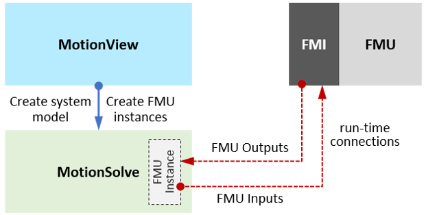
Two versions of the FMI, FMI 1.0 and FMI 2.0, are used today. MotionSolve supports only FMI 2.0.
- The contents of an FMUAn FMU is distributed in a zip file that normally has the extension .fmu. The zip file has the following structure:
- modelDescription.xml
- This is the FMI Model Description File. All static information related to an FMU is stored in this text file XML format. Quantities such as the number of input and output signals, the number of parameters and their attributes, such as name, unit, default initial value and so on, are stored in this file.
- model.png
- An optional image file of the FMU icon.
- sources
- An optional directory containing all C sources. All needed C sources and C header files to compile and link the FMU are included in this directory.
- binaries
- A directory containing the binaries. Binaries are commonly provided if the FMU provider wants to hide the source code to protect confidential information and knowledge. Separate subdirectories are provided for each supported platform. The binaries are typically in the form of dynamic linked libraries (.dll for Windows and .so for Linux)
- resources
- An optional directory, which contains additional FMU data (like tables, maps, and data files) in FMU specific file formats, that the FMU knows how to read.
- Model Exchange FMU (ME-FMU)
This type of FMU only defines the equations and other quantities typically needed for a function evaluation. It does not compute the response of the FMU. Instead, the equations of the FMU are incorporated into the solution scheme of MotionSolve and MotionSolve will simultaneously compute the time history of the evolution of the FMU as the simulation progresses. This is a fully coupled solution. The FMU may contain any combination of ordinary differential equations, algebraic equations, and discrete difference equations. MotionSolve can handle all three types of equations.
The structure of an ME-FMU and how it is included in a system model is shown below.- A system model is being simulated. This is shown as a grey box.
- The system model talks to a solver that computes the response of the model to the inputs that are provided. The solver is shown as a yellow box.
- One or more FMUs are included in the system model. This is shown as a blue box inside the grey box.
- The system model does the following:
- In the very first call, it obtains the user-specified start time t0 and user-specified list of variables known exactly at t0, vstart.
- Obtains the current simulation time t and the FMU continuous states xc from the solver (at t0 the solver just returns the initial value provided by the FMU).
- Computes the state dependent inputs, u.
- Given the above input, the FMU does the following:
- Computes the local variables it needs, w.
- Computes the event indicators, z.
- Computes its outputs, y, and returns it to the system model.
Figure 2. FMU Structure 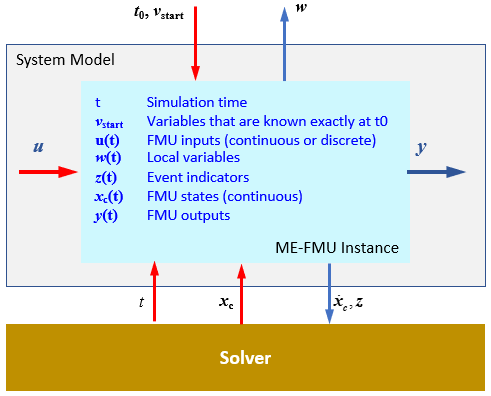
- Co-Simulation FMU (CS-FMU)FMI for Co-Simulation is designed for coupling with subsystem models, which have been exported by their simulators. The FMI is available as follows:
- The FMU solver is embedded in the FMU.
- The FMI is just a wrapper that knows how to talk to an external solver.
Figure 3. Co-Simulation with generated code 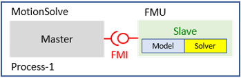
Figure 4. Co-Simulation with tool-coupling 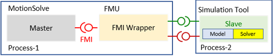
MotionSolve provides the FMU with the necessary inputs and asks the FMU (its embedded solver) to compute its response for a specified time duration. Depending on the implementation, the MotionSolve inputs are interpolated or extrapolated to provide the input signal values at various points in time required by the FMU solver. The embedded solver computes the FMU’s internal states and subsequently the necessary outputs. As the name implies, this is a co-simulation approach.
The FMU may contain any combination of ordinary differential equations, algebraic equations and discrete difference equations. All of these are hidden from MotionSolve and only the outputs are provided to MotionSolve.
- Solver Arrays referenced by an FMUThe model-exchange FMU contains references to four types of Solver Arrays – X, U, Y, IC (optional). The Cosimulation FMU contains references to two types of Solver Arrays – U, Y. These are explained below.
- State array (X):
- A solver Array holds the continuous states of the model-exchange FMU. Inside the FMU, the states, X, are defined through a set of coupled Ordinary Differential Equations of the form:
- Input array (U):
- A solver Array holds the inputs from the FMU. The system model computes the required inputs to the FMU as a function of time and its own internal states. The inputs, U, are defined through a set of coupled Algebraic Equations of the form:
- Output array (Y):
- A solver Array holds the outputs from the FMU. Inside the FMU, the outputs, Y, are defined through a set of coupled Algebraic Equations of the form:
- Initial conditions array (IC):
- A solver Array holds the initial conditions X0 for the FMU states. MotionSolve and the FMU can run either on the same computer or they may run on separate machines. The ip_address attribute is used to specify this. Regardless, MotionSolve uses an inter-process communication protocol to exchange data with the FMU.
- The ip_address
attribute
When MotionSolve and the FMU run in the same machine, ip_address = “PIPE” is the default. This specifies a name pipe that serves as a communication medium between the FMU and MotionSolve.
When MotionSolve and the FMU run in different machines, the IP address of the machine running the MotionSolve is passed to the FMU so it can talk to MotionSolve. For example, ip_address = “172.16.254.1”.
In this case, TCP/IP (Transmission Control Protocol/Internet Protocol) is used. TCP/IP is a suite method used to connect heterogeneous network devices on the internet. TCP/IP can also be used as a communications protocol in a private network. In this scenario, the FMU resides on a different computer and communicates with MotionSolve. The two computers can be in geographically different locations. Two scenarios are possible and both are supported:- MotionSolve and the FMU are on the same machine type (for example, both run on Win64)
- MotionSolve and the FMU are on different machine types (for example, MotionSolve is running on WIN64 and the FMU is on LINUX64, or vice versa).
- FMU analysis support in MotionSolve
The MotionSolve analysis support for FMUs depend on the type of the FMU. The analysis support is summarized in the table below. Analysis modes that are not supported are shaded in salmon color.
Figure 5. Analysis support for FMU in MotionSolve 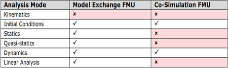
- The is_static_hold attribute
The behavior of the dynamic states associated with the FMU during static and quasi-static solutions is governed by the attribute, is_static_hold.
is_static_hold = "TRUE"
If the solution is done at time T = 0, the states are kept fixed at the value specified by the IC array. If the solution is being done after a dynamic analysis, then the value is kept fixed at the last value obtained from a dynamic simulation.
The equations defining the continuous states for the FMU are replaced with the following: x(t*) = x*, where x* is a constant.
Note: When the dynamic states are kept fixed, their time derivatives no longer are zero at the end of the static equilibrium or a quasi-static step. The inputs u will have changed. This may lead to transients in the solution if a dynamic solution were to be subsequently performed.is_static_hold = "FALSE"
The states are not kept constant but allowed to change as the configuration of the entire system changes during the solution process. Here is how this is accomplished:- For static and quasi-static solutions, the derivative of the dynamic states is set to zero. This converts the FMU to a set of algebraic equations for these two analyses.
- During the equilibrium solution, the input u changes as the system changes its configuration to meet the equilibrium conditions. The above equations are solved to compute x for the current value of u.
- This method ensures that the time derivative of the dynamic states is zero at the end of the static or quasi-static solution and ensures a smooth subsequent dynamic analysis.
- The error_tol_factor
attribute
The error_tolerance_factor attribute is used only when the FMU type = “ModelExchange”.
The error_tol_factor is used to control the accuracy of the continuous states in an FMU. The displacement integration error tolerance is multiplied by this factor to compute the integration error tolerance for the FMU’s continuous states.
error_tol_factor = 0.5 implies that the FMU states have an error tolerance that is twice as strict as the error tolerance for the displacement states in the model.
Similarly, error_tol_factor = 2.0 implies that the FMU states have an error tolerance that is twice as loose as the error tolerance for the displacement states in the model.