
Reference: Solver Variable
Model ElementReference_Variable defines an algebraic state in MotionSolve.
Description
- Directly as an explicit function of system state and time.
- Directly as an implicit function of system state and time.
- Indirectly through an algebraic equation applied as a constraint or a penalty.
- As the integral of an expression.
Reference_Variables are quite versatile and have many different applications in modeling multibody systems. They are used to create signals of interest in the simulation. The signal may then be used to define forces, create independent variables for interpolation into test data, define inputs to generic control elements, and create complex output signals.
Format
<Reference_Variable
           id                   = "integer"
          [label                = "string"]
        {
           type                 = "EXPRESSION"
           expr                 = "motionsolve_expression"

           type                 = "USERSUB"
           usrsub_dll_name      = "valid_path_name"
           usrsub_fnc_name      = "custom_fnc_name"
           usrsub_param_string  = "USER(par_1, ..., par_n)"

           type                 = "USERSUB"
           script_name          = "valid_path_name"
           interpreter          = "string"
           usrsub_fnc_name      = "custome_fnc_name"
           usrsub_param_string  = "USER(par_1, ..., par_n)"

        }
        [[
           is_implicit          = "true" | "false"
           autobalance          = "default" | "conditional" | "disabled" | "penalty"

           penalty              = "double"
           penalty1             = "double"

           dot_form             = "true" | "false"
           [[ic = "real"                   ]]
           [[static_hold = "true" | "false"]]
        ]]
/>
Attributes
- id
- Specifies the element identification number (integer>0). This number is unique among all Reference_Variable elements.
- label
- This attribute describes the name of the Reference_Variable element. The description is primarily used to make the input more readable.
- type
-
Select from EXPRESSION and USERSUB. Specifies how the variable expression is defined.
- The EXPRESSION option specifies that the value of the Reference_Variable is a MotionSolve expression that can be evaluated at run-time.
- The USERSUB option indicates that the value of the event is specified in a user-defined subroutine. Parameters "usrsub_param_string" and "usrsub_dll_name" are used to provide more information about the user-defined subroutine.
- expr
- Specifies the MotionSolve expression that defines the Reference_Variable. Use this parameter only when type= EXPRESSION. Any valid run-time MotionSolve expression can be provided as input.
- usrsub_dll_name
- Specifies the path and name of the DLL or shared library containing the user subroutine. MotionSolve uses this information to load the user subroutine in the DLL at run time. Use this keyword only when type = USERSUB.
- usrsub_fnc_name
- This parameter allows you to specify the name for the user subroutine. The default name, VARSUB, is used when the attribute is not specified. Use this keyword only when type = USERSUB.
- usrsub_param_string
- The list of parameters that are passed from the data file to the user- defined VARSUB. Use this keyword only when type = USERSUB.
- script_name
- Specifies the path and name of the user written script that contains the function specified by usrsub_fnc_name. Use this keyword only when type = USERSUB.
- interpreter
- Specifies the interpreted language that the user script is written in (example: "PYTHON"). See User-Written Subroutines for a choice of valid interpreted languages.
- is_implicit
- By default, all Reference_Variables are explicitly specified. This keyword is used to indicate that the variable is defined implicitly. For more information about this, please refer to Comments 2 and 3.
- auto_balance
-
This attribute tells MotionSolve how to deal with the Lagrange Multiplier in the case where a variable defines an algebraic relationship.
- "Conditional" means that MotionSolve is to implement a hard constraint, and Lagrange Multipliers are to be calculated as a part of the solution process. The resulting constraint reaction forces and torques, due to the Lagrange Multiplier, are automatically applied except when finite differencing is performed within GTCMAT.
- "Unconditional" means that MotionSolve is to implement a hard constraint, and Lagrange Multipliers are to be calculated as a part of the solution process. The resulting constraint reaction forces and torques, due to the Lagrange Multiplier, are automatically and unconditionally applied without exceptions.
- "Disabled" means that MotionSolve only implements the constraint equation. Generalized reaction forces due to the Lagrange Multipliers are not applied to the equations of motion. You have to do this by applying equivalent forces.
- "Penalty" means that MotionSolve implements the constraints using a penalty formulation. For more information, see Comment 3.
The default behavior of MotionSolve is "conditional".
- penalty
- Used only when auto_balance=penalty. Specifies a penalty factor to be used in calculating the restoring force that is used to enforce the constraint. See Comment 3 for more details.
- penalty1
- Used only when auto_balance=penalty. Specifies a second penalty factor to be used in calculating the restoring force that is used to enforce the constraint. See Comment 3 for more information.
- dot_form
- Specifies that the integral of the value defined in expr is to be used as the value of the Reference_Variable.
- ic
- Should be used only when dot_form = "True". When a Reference_Variable is defined in integral form, it requires an initial value. Use the IC attribute to specify an initial value for a Reference_Variable. IC defaults to 0 when it is not specified.
- static_hold
- Should be used only when dot_form = "True". Static_Hold specifies that value of the Reference_Variable is to be kept fixed to the IC value during static equilibrium iterations. When not specified, MotionSolve will change the initial value of the variable as needed.
Example 1
This example demonstrates how to use an EXPRESSION based Reference_Variable to calculate the kinetic energy of a rigid body. In the example below, the ID of the Reference_Variable is 3070. 1011 is a MARKER that defines the center of mass of a rigid body with mass 4kg and principal moments of inertia Ixx=0.006 Kgm2, Iyy=0.005 Kgm2, and Izz=0.004 Kgm2. Reference_Variable 3070 is the total kinetic energy of the rigid body.
<Reference_Variable
   id    = "3070"
   type  = "EXPRESSION"
   expr  = "0.5*(4*VM(1011)**2 + 0.006*WX(1011)**2 + 0.005*WY(1011)**2 + 0.004*WZ(1011)**2)"
/>
Example 2
The second example does the same as the first example. The implementation, however, is done within a user subroutine. A user-defined subroutine VARSUB that can calculate the Kinetic Energy of any rigid body is written first. The input parameters to the VARSUB are the mass and inertia properties of the rigid body and the ID of the center of mass Marker. The VARSUB returns the kinetic energy of the rigid body. This provides a generic function that can calculate the kinetic energy of any rigid body.
<Reference_Variable
    id                  = "3070"
    type                = "USERSUB"
    usrsub_param_string = "USER (1011, 4, 0.006, 0.005, 0.004)"
    usrsub_dll_name     = "/Users/ms_test/ke.dll"
    usrsub_fnc_name     = "Kinetic_Energy"
/>
The VARSUB, written in Python, is shown below.
from math import *
def VARSUB(id, time, par, npar, dflag, iflag):
    # Get information from the par array
    icm     = 1*[0]
    icm[0]  = par[0]
    mass    = par[1]
    ixx     = par[2]
    iyy     = par[3]
    izz     = par[4]

    # get the translational and rotational velocity states
    [vm,errflg] = py_sysfnc ("VM", icm)
    [w, errflg] = py_sysary ("RVEL", icm)

    # Calculate the kinetic energy
    if iflag:
        KE = 0.0
    else:
        KE = 0.5 * (mass*vm**2 + ixx*w[0]**2 + iyy*w[1]**2 + izz*w[2]**2)

    return KE
Example 3
The third example demonstrates a simple 2D example where a constraint is applied at one point in the system but the reaction forces are desired at some other point. Figure 1 represents a 2D robot that is anchored to ground. The end-effector of the robot, T, is required to trace a path in 2D space as shown in the figure. F(t) and g(t) are specified through Spline/1 and Spline/2, respectively. The parameter t represents system simulation time. In the model, Reference_Marker 11 represents the tip of the end-effector.
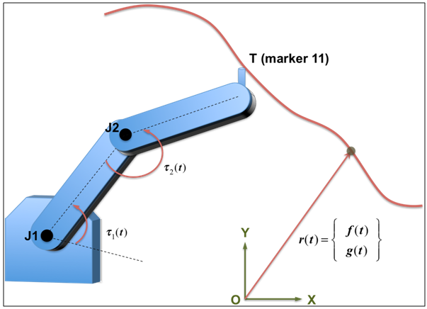
The various bodies have mass and inertia properties and they have a well-defined geometry. For the purposes of this example, they are not relevant. However, it is important to note that they have to be defined elsewhere in the model.
As a designer of the robot, you are required to size the motors acting at revolute joints J1 and J2 in the system. In order to size the motors, you need to know the torques that are to be applied at the joints. If you create three Motion_Markers to define the constraints, MotionSolve will compute the forces at the tip of the end-effector, not the torques that are to be applied at J1 and J2.
- Define two algebraic constraints that define the motion of Marker
11
<Reference_Variable |<Reference_Variable id = "1" | id = "2" type = "EXPRESSION" | type = "EXPRESSION" expr = "DX(2011) - cubspl(time, 0, 1)" | expr = "DY(2011) - cubspl(time, 0, 2)" is_implicit = "True" | is_implicit = "True" autobalance = "Disabled" | autobalance = "Disabled" /> |/> - Apply the internal force as torques at joints J1 and J2
Assume that J1 is defined with I marker=33, J Marker=44 and J2 is defined with I marker=55, J Marker=66. Assume also that the ground coordinate system is represented with marker ID = 77.
<Force_Vector_TwoBody | <Force_Vector_TwoBody id = "1" | id = "2" type = "TorqueOnly" | type = "TorqueOnly" i_marker_id = "33" | i_marker_id = "55" j_floating_marker_id = "44" | j_floating_marker_id = "66" ref_marker_id = "77" | ref_marker_id = "77" tx_expression = "0" | tx_expression = "0" ty_expression = "0" | ty_expression = "0" tz_expression = "VARVAL(1)" | tz_expression = "VARVAL(2)" /> | /> - Look at the torques applied at the Joints to size the motors
Varval(1) and Varval(2) are the torques applied at joint J1 and J2 respectively.
Example 4
This example demonstrates the use of Reference_Variables to define Plant_Inputs for a control system defined in MATLAB. Consider the control problem of stabilizing an inverted pendulum mounted on a slider. The image below shows one such setup. The slider, the green block, is constrained to move along the global X-axis by a translational joint with ground, depicted as the red strip.
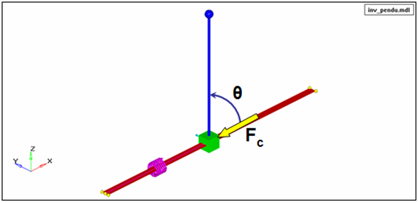
- Plant input: Control force Fc acting on slider. This is computed by MATLAB and sent to MotionSolve.
- Plant output: Pendulum angle θ and angular velocity ω. These signals are sent to MATLAB.
The plant output may be defined as follows:
<Control_PlantOutput
   id                = "303001"
   num_element       = "2"
   variable_id_list  = "12", "13"
   hold_order        = "1"
/>
Reference_Variable 12 defines the pendulum angle θ and Reference_Variable 13 defines the pendulum angular velocity, ω. These Reference_Variables are defined below.
<Reference_Variable         |<Reference_Variable
  id    = "12"              |  id    = "13"
  type  = "EXPRESSION"      |  type  = "EXPRESSION"
  expr  = "-AY(1011,2011)"  |  expr  = "-WY(1011,2011)"
/>                          |/>
Example 5
This example illustrates a variable used to define a steering gear ratio in an automobile model. The Steering Ratio is the ratio between the turn of the steering wheel and the turn of the wheels. A higher steering ratio means that you have to turn the steering wheel more to get a specific wheel turn, but it will be easier to turn the steering wheel. A lower steering ratio has the inverse effect.
The objective of this exercise is to use a Reference_Variable to define the steering ratio, given the steering when angle. Once the ratio is defined, it can be used downstream to apply the correct torques on the wheels.
Assume that the revolute joint on the steering wheel is defined by I-Marker = 6565 and J-Marker = 7676. The variables defining the steering angle and the steering gear ratio are shown below.
<Reference_Variable                      | Reference_Variable
  id    = "1"                            |  id    = "2"
  label = "Steering angle in degrees"    |  label = "Steering gear ratio"
  type  = "EXPRESSION"                   |  type  = "EXPRESSION"
  expr  = "RTOD * ABS(AZ(6565,7676))"    |  expr  = "step(varval(1), 100, 1000, 150, 1500)"
/>                                       | />
Example 6
A Reference_Variable may be used to define a "soft constraint" by using the penalty option. Here is a simple example to illustrate this.
Consider a situation where you want to maintain the angle between the z-axis of Marker 11 and the z-axis of Marker 21 to be 60 degrees as shown in Figure 4 below.
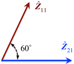
You could use a General_Constraint to define this constraint. However, if you wanted to include some system flexibility in the model, then you would want to model the kinematic condition as a "soft constraint", so as to allow some violation.
<Reference_Variable | The torque that is implemented
id = "1" |
label = "A soft constraint" |
type = "EXPRESSION" |
expr = "theta(21,11) - 60D |
is_implicit = "TRUE" |
autobalance = "PENALTY" |
penalty = "1000.0" |
penalty1 = "10.0" |
/> <Force_Penalty | The torque that is implemented
id = "1" |
label = "A soft constraint" |
type = "EXPRESSION" |
expr = "theta(21,11) - 60D" |
penalty = "1000.0" |
penalty1 = "10.0" |
/>Comments
- Direct, explicit variables are defined as follows: varval = g(y,t). varval is the value of the variable, and y is any set of system state dependent values. The expression or user subroutine defines the function g(y,t).
- Direct, implicit variables are defined as follows: g(varval,y,t)=0. Once again, varval is the value of the variable, and y is any set of system state dependent values. The expression or user subroutine defines the function g(varval, y,t). Note, for this type of variable, varval must be explicitly referenced in the function g(...).
- Algebraic constraints are defined as follows:
g(y,t)=0. y is any set of system state
dependent displacement values. The expression or user subroutine defines the
function g(y,t). Note, for this type of
variable, varval is never explicitly referenced in the
function g(...). varval is a Lagrange Multiplier. It
represents the internal force required to maintain the constraint
g(y,t)=0.
g(y,t)=0 may be applied as a hard
constraint. In this case, varval is a system unknown and is
determined by MotionSolve. Alternatively,
g(y,t)=0 may be applied as a "soft"
constraint via penalty functions. In this case, varval
returns the constraint value g(y,t) and this
constraint violation is neither enforced nor monitored by MotionSolve. An artificial Lagrange Multiplier is
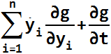
calculated as -penalty*g(y,t)-penalty1*ġ(ẏ,y,t), where ġ(...) =
 ,
and the resulting constraint reaction forces and torques, due to this Lagrange
Multiplier, are automatically applied to the multibody system. For more
information on auto_balance=penalty, see Force_Penalty.
,
and the resulting constraint reaction forces and torques, due to this Lagrange
Multiplier, are automatically applied to the multibody system. For more
information on auto_balance=penalty, see Force_Penalty. - Variables can be defined in integral form as follows:
ż = g(y,t); varval = z. varval is the value of the variable (which is the integral of g(y,t)), and y is any set of system state dependent values. The expression or user subroutine defines the function g(y,t).
- Three approaches are available for defining the function
g(y,t).
- As a function expression in the XML file: This is probably the simplest approach, and g(y,t) is defined as an expression composed from the built-in functions and operators in the function expression language.
- As a compiled user-written subroutine, provided in a DLL: Any language may be used. MotionSolve provides an interface to Fortran, C and C++. The default name for the user-written subroutine is VARSUB. However, you are allowed to give the function any name and tell MotionSolve what it is.
- As a script written in Python or Matlab: Though this approach is less efficient than writing the user-written subroutine in a compiled language, it provides two significant benefits: (A) It provides for a vastly more flexible and powerful environment to compose the the function g(y,t) than function expressions, and, (B) There is no need for compilers and linkers as is the case when Fortran, C or C++ are used.
- Recursive definitions of variables are not allowed when the integrator is ABAM, VSTIFF, or MSTIFF.
- In the MotionSolve input language, Reference_Variables are used to define the following elements: Control_PlantInput, Control_PlantOutput, and Reference_Array.
- In general, we do not recommend using Reference_Variable in function expressions for defining MOTION modeling elements.
- The user-subroutine, VARSUB, may be used to define discrete algebraic states. In other words, states that change only at specific sample times. However, you need to implement the logic for managing the sampling and update actions within the user-defined subroutine.